A STEP-BY-STEP GUIDE FOR LEARNING
AND GETTING FAMILIAR WITH GPS-X

GPS-X Version 8.0
A STEP-BY-STEP GUIDE FOR LEARNING
AND GETTING FAMILIAR WITH GPS-X
GPS-X Version 8.0
Copyright ©1992-2019 Hydromantis Environmental Software Solutions, Inc. All rights reserved.
No part of this work covered by copyright may be reproduced in any form or by any means - graphic, electronic or mechanical, including photocopying, recording, taping, or storage in an information retrieval system - without the prior written permission of the copyright owner.
The information contained within this document is subject to change without notice. Hydromantis Environmental Software Solutions, Inc. makes no warranty of any kind with regard to this material, including, but not limited to, the implied warranties of merchantability and fitness for a particular purpose. Hydromantis Environmental Software Solutions, Inc. shall not be liable for errors contained herein or for incidental consequential damages in connection with the furnishing, performance, or use of this material.
Trademarks
GPS-X and all other Hydromantis trademarks and logos mentioned and/or displayed are trademarks or registered trademarks of Hydromantis Environmental Software Solutions, Inc. in Canada and in other countries.
ACSL is a registered trademark of AEgis Research Corporation
JAVA is a trademark of Oracle Corporation.
Python is a registered trademark of the Python Software Foundation.
Microsoft, Windows, Word and Excel are trademarks of Microsoft Corporation.
GPS-X uses selected Free and Open Source licensed components. Please see the readme.txt file in the installation directory for details.

Table of Contents
Why Create Models of Wastewater Treatment Plants?
Building a Simple Plant Layout
Editing Layouts and Using Scenarios
Generating Records of Model Dependent and Independent Variables
Creating a New Output Table Tab
Creating a Mass Balance Diagram
Viewing an Energy Usage Summary
Viewing an Operating cost Summary
Influent Data & Influent Advisor
Plotting Measured Data along with Simulated Results
Statistical Analysis of the Models Performance
Creating a Bar Chart for Steady-State Condition
Using an Automatic DO Controller
Using an Automatic MLSS Controller
Controlling SRT with Waste Pump Rate
Setting up the Analysis Parameters
Automatic Calibration Using the Optimizer
Adding Custom Output Variables
Setting Up Simulations with Custom Variables
Dynamic Parameter Estimator (DPE)
GPS-X with Python - Introduction
GPS-X and Python – Basic Simulation
GPS-X with Python – Random Events
GPS-X with Python – Sensitivity Analysis
Two Manipulated Variable Sensitivity Analysis
Multi-Variable Sensitivity Analysis
GPS-X with Python – Java Classes
Using JARS to Create Real Time Plots
GPSX With Python – DDO Optimization
Creating an Objective Function
GPS-X is a software tool that allows for the mathematical modeling, simulation, optimization, and management of wastewater treatment plants. It uses a simple drag and drop interface and comprehensive selection of unit processes to allow for users to simply develop a plant model, enter in characterization data, and run simulations.
Models are most commonly implemented to “stand-in” for a real plant process, when testing and analysis on the actual plant is not available or feasible. The five primary reasons are as follows:
1. Allow for the comparison of various designs, process retrofits or operating strategies
Here users can simply adjust a plant design through the adjustment and/or addition of unit processes. For instance, modelling could be used to determine the sizing of the anoxic, and aerobic zones in an IFAS bioreactor to achieve a particular level of effluent quality.
2. Verify the capacity of the existing plant
For a plant experiencing higher influent flows due to surrounding population growth, a model of the plant could be run at increasing flow rates to determine the flow rate at which the plants effluent quality or design capacity would be theoretically exceeded.
3. Determine process bottlenecks
A plant model could allow for identification of which operational units are causing overall plant performance. For instance, it could help identify if the secondary clarifier wastage rate was too low, resulting in sludge buildup in the clarifier and higher TSS concentrations in the effluent.
4. Identify strategies to allow for enhanced cost savings
Many plants are operated in a conservative manner to limit the potential for poor effluent quality. While it is extremely important to maintain good treatment of wastewater, some practises can lead to an excessive use of energy. For example, through the use of modelling, it could be determined that a plant could be operated at a DO setpoint of 1.4 mg/L rather than 2 mg/L allowing for huge energy savings and negligible change in the effluent water quality.
5. Support regulatory decision making
Wastewater treatment plants are responsible for reporting to regulatory bodies. In cases where an effluent limit was exceeded they may need to provide a reasonable explanation for the cause of the exceedance. For instance, using a simulation model could help determine that consistently low winter temperatures were responsible for TAN breakthrough in the effluent.
Before moving forward with the tutorials, take a moment to familiarize yourself with the GPS-X Version 8.0 interface. This introduction will provide a basic tour of the interface, allowing new users to become more comfortable with the layout, prior to building and running plant model simulations.
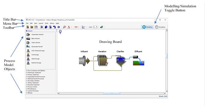
Once GPS-X is opened, observe the basic elements of the GPS-X interface. Make note that you are in Modelling Mode and the button at the top-right of the window can be used to switch between Modelling Mode and Simulation Mode.
Located here is information regarding the version of GPS-X being used, the name of the model layout being edited, and the library that the layout is using.
Here there are several menus available:
1. File: Contains items for file handling and manipulation. Additionally, users can access sample layouts, including those for the tutorials, create a zip folder of all files associated with the model layout, and view historical model layouts.
2. Edit: allows users to manipulate objects on the drawing board such as cutting and pasting an object or rotating it.
3. View: allows users to adjust the look of the drawing board and how model objects are being displayed.
4. Layout: allows the user to specify global simulation properties, customized user-code and common plant-wide properties.
5. Tools:allows access to items relating to the setup and use of a plant model.
6. Library: provides access to a list of available libraries in GPS-X. Please access the Technical Reference Manual for more information.
7. Help: Under Help>Manuals, users can reference 5 documents relating to GPS-X. These should be referred to first when troubleshooting or learning how to use the software. By selecting
The buttons in this section allow for quick access to particular functions in GPS-X. All of these functions are found in the menus presented in the menu bar.
These are the available model objects that can be used to construct the plant models. These are divided into subsections based on their function. For example, under the Suspended Growth Processes header, users can locate objects for a CSTR, plug-flow tank, and a membrane bioreactor.
This large white space is where the model objects are arranged to construct a plant model.
Using the button at the top-right of the screen you can switch into Simulation Mode. Observe the basic elements of the interface.

Here users can create controllers for specific plant properties. For example, shown above are controllers for the influent total carbonaceous BOD, total TKN and influent flow, as well as some process control variables. These allows users to have quick access to variables to be adjusted during a model simulation.
This space contains a copy of the plant model. Here users can access all of the same menus that are available in Modelling Mode.
This area contains the output graphic displays. Automatically tabs are created for each model object, and users have the opportunity to develop their own custom tables and graphs to display key characteristics of interest.
Once a simulation is run, users have access to buttons to export results, display mass and flow rates on the plant schematic (Sankey and Mass Balance Diagrams), and observe the Energy Usage Summary and Operating Cost Summary information.
Here users can run the plant simulations. There are Play, Continue, and Pause buttons, and the bar allows for users to see the extent of convergence when the simulation is running. Additionally, within this toolbar, users can create customized scenarios that allow for adjustment of specific model properties.
The subsequent tutorials contained within this manual will provide an in-depth exploration of the GPS-X interface and features available in this software. Tutorials 1 – 8 should be completed if you are new to using GPS-X, while the remaining tutorials cover specific topics that may not be applicable for every user.
Dynamic process models have great potential for assisting operators, engineers and managers. However, in the past dynamic models were not used very often because the cost of building models, running simulations and interpreting the results were too expensive. In order to simplify the modelling process and therefore reduce costs, you need tools to aid you with the steps in any modelling exercise.
A tool like GPS-X is invaluable as its easy-to-use interface connected to a powerful library of simulation models will greatly reduce the expense of carrying out simulation studies.
There are five major steps in any modelling study:
1. Model construction
2. Model calibration
3. Scenario development
4. Simulation
5. Interpretation of results
In this tutorial, you will develop and simulate a simple steady state model of an activated sludge system.
This tutorial covers the following topics:
1. Gaining familiarity with the GPS-X interface and the tools available
2. Building a simple plant layout
3. Running a simple simulation
When you have finished this tutorial, you will be able to build a process layout in the modelling environment and then simulate it in the simulation environment. This provides a supporting basis for the subsequent tutorials where you will learn how to create interactive controls and output graphics
After opening a new file in GPS-X:
Select the Comprehensive – Carbon, Nitrogen, Phosphorus, pH (mantis2lib) from the Library menu (if it isn’t already selected).
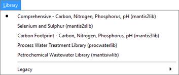
Figure 1‑1 - Select Library
1. Locate the Process Table on the left-hand side of the GPS-X window. These icons are used to build a plant layout. Icons represent the unit processes and control points in a layout. The icons are separated into groups of like objects, such as Preliminary Treatment, Suspended Growth Processes, and Biosolids Treatment.
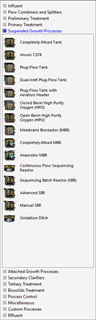
Figure 1‑2 – Process Table
The Process Table contains the unit process icons used to construct a treatment plant model. Each icon is identified by process name. The process name is also displayed in a tooltip if you hold the cursor over any object in your drawing board.
We will start by building a simple wastewater treatment plant consisting of 4 objects:
· A secondary clarifier
· A Wastewater Outfall
|
|
2. Place the Wastewater Influent object on the drawing board. If the Influent group is not selected in the process table, click on the Influent process group to display the influent process objects. Place the cursor over the brown arrow influent object. Click on the left mouse button and with the button pressed, drag the cursor to the center of the drawing board and drop the object by releasing the mouse button. The influent object now appears in the drawing board. You can drop as many of these objects as desired by repeating this procedure. For now, drop only one influent object. |
|
|
3. Select the Plug-Flow Tank icon (Suspended Growth processes group) and drop it on the drawing board to the right of the influent object. |
|
|
4. Select the Circular Secondary Clarifier icon (Secondary Clarifiers processes group) and it to the right of the plug flow reactor. |
|
|
5. Select the Wastewater Outfall icon (Effluent group) and drop it to the right of the circular secondary clarifier. |
|
|
6. (Optional) Close the Process Table by clicking on the left-pointing arrow at the top-right corner of the Process Table or by going to View > Toolbars > Process Table from the main menu. |
The drawing board should now look similar to the Figure 1‑3.
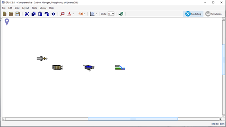
Figure 1‑3 – Drawing Board with 4 Unit Processes
|
|
7. Zoom in by using the Locator. This is a simple plant with a large amount of white space on the drawing board, and zooming will allow us to see the objects on the drawing board more clearly. The Locator can be used to zoom in on an area of interest while leaving white space for additional objects. The Locator can be accessed by going to View > Zoom. The Locator window will be displayed as shown in Figure 1‑4. |
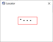
Figure 1‑4 – Locator Window
8. Zoom in or out by selecting a region in the Locator window (left-click, drag and release). Try selecting an area much larger than the rectangle currently displayed in the Locatorwindow. When you release the mouse button the drawing board is refreshed and the icons on the drawing board appear smaller. Try dragging-out a smaller rectangle around the process units and note the effect in the main drawing board area. You should see an enlarged view like that shown in Figure 1‑5.
|
Alternatively, the mouse wheel can also be used to zoom in and out on the layout. |
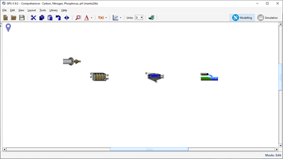
Figure 1‑5 – Enlarged Drawing Board Area
|
|
9. Zoom in by using the Zoom to selection/plant. The Zoom to selection/plant button located on the main toolbar will automatically adjust the current level of zoom to fit all objects on the drawing board.
This functionality can also be used to automatically zoom in on a specific region of the plant. This can be done by clicking and dragging the blue box around the area of interest. Pressing the Zoom to selection/plant button will zoom in on the highlighted area to fill the drawing board. |
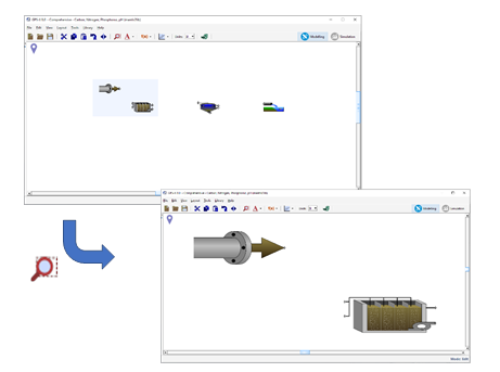
Figure 1‑6 - Using Zoom to Selection/Plant to Zoom on a Region of Interest
Press the Zoom to selection/plant button to obtain the enlarged view of the entire plant again.
10. Specify the connectivity between the objects. This is critical in the specification of a flow sheet as all material balances, and therefore the equations which result, are based on the connectivity in the layout. When you specify these connections, remember that the flow lines are directional, i.e., materials flow from the initial point to the terminal point of the flow connection.
|
|
To specify the connectivity between objects, in the drawing board, move the pointer over the influent object connection point. You will know that you are over the connection point when the mouse pointer changes from the default `Windows' arrow to a connecting arrow. When the connecting arrow appears, click to anchor the flow line at this initial point. |
Next, drag the pointer from the influent object to the influent connection point of the plug flow tank (top left hand corner of the icon, NOT the return flow connection point just below on the left-hand side of the icon). When the connecting arrow re-appears, release the mouse button. A connecting pipe will be drawn between the influent object and the plug-flow tank.
In a similar manner, connect the effluent point from the plug-flow tank (top right hand corner of the icon) to the secondary clarifier.
Connect the underflow from the secondary clarifier (bottom of the secondary clarifier icon) to the return flow point of the aeration tank (lower left hand corner of the plug-flow tank icon).
Finally, connect the effluent overflow in the secondary clarifier (top right hand corner of the icon) to the Wastewater Outfall connection point.
In this example, excess sludge will be wasted from the bottom of the secondary clarifier (lower right hand corner of the clarifier icon). As this model does not consider any downstream processing of the excess sludge, it is not necessary to specify a flow connection from this point (see Figure 1‑7).
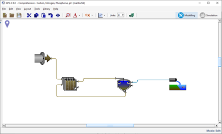
Figure 1‑7 – Specifying Connectivity
|
NOTE: GPS-X does not allow invalid flow connections. For example, flows which initiate at the influent of an object and terminate at the influent of a second object are not allowed. GPS-X will disallow an incorrect connection by displaying an invalid sign. If you experience some difficulty in specifying flow connections, you can delete the flow lines by right-clicking on the flow line and selecting Delete Connection |
|
|
11. Rearrange the Connections. The path that a flow line takes from the initiation to termination point can be moved by placing the cursor over the flow line until the mouse icon changes from the default ‘Windows’ arrow to a double ended arrow icon and the connection turns red. Selecting a horizontal segment of the connection will allow you to adjust its path up and down while selecting a vertical segment will allow you to move the flow left and right. |
If you would like to specify a corner point on a flow line, right-click the flow line at the point of interest and select Create Breakpoint from the menu. This will separate the line into two independently moving segments. The break point will stay in place while you modify the other segments.
Try adjusting the flow paths until you are happy with the design of the drawing board. If you would like to revert a connection line back to the GPS-X default path, right-click the connection and select Reset to Auto-Draw from the menu.
12. Show or re-name the labels. There are two types of labels. The unit processes themselves have optional labels and the streams (ie. the flow lines) each have labels. The stream labels are initialized to incremental numbers when a unit process is dropped onto the drawing board.
|
|
In the completed layout shown in Figure 1‑7 there are numbers associated with each of the flow streams. To show/hide these labels on the drawing board, press on the Labels button on the main toolbar to open a dropdown menu where you can specify if you would like to display the Stream and Object labels. |
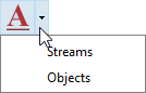
Figure 1‑8 – Labels Submenu
Note that the processes that you currently have on the board do not yet have labels, so showing/hiding the Objects label will have no effect at this time.
To change the labels, right-click on an object icon and the process data menu will be displayed. Select the Labels… item from this menu as shown in Figure 1‑9.
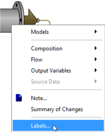
Figure 1‑9 - Process Menu showing Labels item
New label names can be entered to the form that is displayed in Figure 1‑10. Save these changes by choosing Accept.
If there is a conflict between your label assignments and existing labels, a Labels Error message will be displayed.
Since GPS-X uses label names to construct variable names in the model, it is important to type label names exactly as shown below in, Figure 1‑10, Figure 1‑11, Figure 1‑12, and Figure 1‑13. for the purposes of this tutorial.
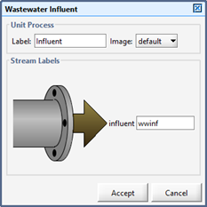
Figure 1‑10 - Influent Labels
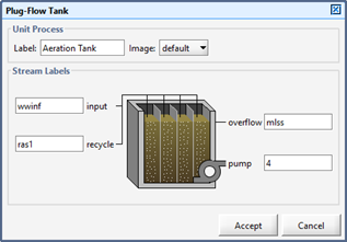
Figure 1‑11 - Plug Flow Tank Labels
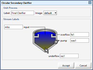
Figure 1‑12 - Clarifier Labels
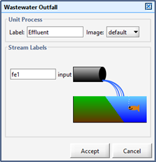
Figure 1‑13 - Wastewater Outfall Labels
|
NOTE: Variable names in GPS-X models use the connection labels to identify a particular stream (e.g. qwwinf for the influent flowrate, and qfe1 for effluent flowrate in this case). These variable names are displayed on some of the forms you will see as you progress through the tutorial chapters. |
|
|
The plant layout is now ready! If you experienced some difficulty in selecting or placing the objects in this layout, you can delete objects from the drawing table by selecting the object (a light blue box will appear around the object) and then pressing Delete on your keyboard. Alternatively, you can always discard the current drawing board and click on the New button to start over again. |
In the previous section, we selected the basic objects to be modeled in our plant. These objects are the major unit processes and control points only. No mathematical models were assigned to the various objects in the layout.
Each object in the layout has a number of attributes or properties, and each attribute has a certain value. One of the most important attributes for GPS-X objects is the set of equations (or model) that defines the dynamic behavior of that object. Remember to distinguish between an object type and the model for that object as some objects have more than one possible model. Each object is given a default model when it is dropped on the drawing board, but these model choices should be verified and changed if required before proceeding.
13. Verify the influent model. Right-click on the influent icon. The process data menu appears as shown in Figure 1‑14. Verify that the codstates item is selected under the Models menu.
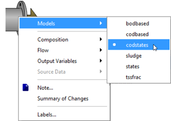
Figure 1‑14 - Selecting Models
14. Verify the plug flow tank model by repeating this procedure on the plug flow tank object. In this case, the only model available should be mantis2.
15. Verify the secondary clarifier object model by making sure that the simple1d (non-reactive 1-dimensional clarification model) item[1] is selected.
16. Verify the wastewater outfall object model by making sure that the default model is selected. This is the only model available for the wastewater outfall.
17. Save the layout. Go to the Filemenu, and select the Save As… menu item. Use the file browser to save the layout to an appropriate directory and with an appropriate name (eg. tutorial-1).
You may have noticed that a process unit object's process menu contains a number of items for specifying other attributes of an object, such as the Input Parameters, Initial Conditions, and Output Variables dropdown menus which are available when right-clicking on a process unit on the drawing board.
In this tutorial, we will use the default properties for the objects you have selected with four exceptions:
· The Influent Total COD Concentration
· The Influent Total TKN Concentration
· The Excess Sludge Wastage Rate
18. Change the influent composition by right clicking on the influent object, move to the Composition sub-menu and select Influent Characterization. A data entry form called Influent Advisor will be displayed.
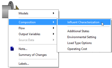
Figure 1‑15 - Accessing Influent Characterization
Change the total CODentry from 430 to 380 gCOD/m3, and the total TKN entry from 40 to 35 gN/m3 as shown in Figure 1‑16.
Note that the values are now highlighted in blue, to indicate that they have been changed from the GPS-X defaults. For more information about the Influent Advisor see Tutorial 5 and Chapter 3 in the GPS-X User’s Guide.
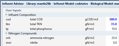
Figure 1‑16 - Change Influent Characteristics
After making the changes, press the Accept button.
19. Change the secondary clarifier wastage rate by right-clicking on the clarifier object, move to the Input Parameterssub-menu and select Operational. A data entry form will appear be displayed.
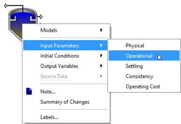
Figure 1‑17 - Accessing Operational Parameters
Change the pumped flow entry from 40 m 3 /d to 60 m3/d.
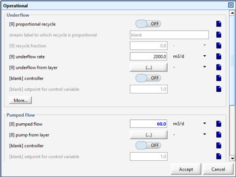
Figure 1‑18 - Change Clarifier Pumped Flow
Once you have changed this flow, press the Accept button.
|
|
20. Once you’ve completed the layout, you’ll usually want to edit some of the plant wide properties. You can access these properties by pressing the Site Properties button on in the upper left corner of the drawing board. A window will be displayed in which you can specify additional details for the plant and make notes about the model. To modify plant wide properties, selecting the Plant Wide Properties tab. Alternatively, you can access these by going to Layout > Plant Wide Properties. For this example, specify the liquid temperature to 22°C. |
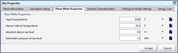
Figure 1‑19 - Plant Wide Properties Window
Press Accept to save the changes.
21. To see all the variables in an object that have been modified from the GPS-X default settings, right-clicking on the object and select the Summary of Changes from the Default option. Verify the changes made to the influent object.
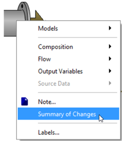
Figure 1‑20 - Accessing Summary of Change
The new form will reflect any changes made specifically to the influent object. Currently it shows the changes made to total COD concentration and total TKN concentration.
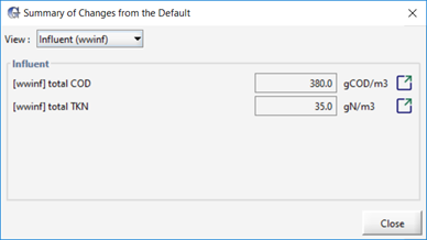
Figure 1‑21 - Summary of Changes made to the Influent Object
By using the drop-down View menu, you can select other objects on the drawing board to see a summary of the changes made to that object. Selecting the System option will display any changes to the models operating conditions, as well as the plant wide properties. Currently this menu shows the changes made to the liquid temperature.
|
|
The Go to location button can be used to be taken directly to that variable’s entry field to make any desired changes. For both variables on the influent object window, this will take you to the influent advisor window. |
22. Save the layout again by clicking the Save button on the toolbar.
Now that you have built a plant layout, the next step is to translate the ‘definition’ of the plant layout and the model parameters, into a model that can run a simulation.
23. Switch from Modelling Mode into Simulation Mode by pressing the Simulation button (Figure 1‑22) in the upper-right corner of the main window.
![]()
Figure 1‑22 – Modelling/Simulation Mode Buttons
This starts the process of compilation and linking, resulting in the creation of an executable model. The time required to complete this process depends on the speed of your workstation, and the complexity of the model.
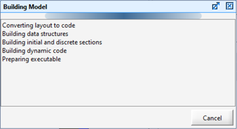
Figure 1‑23 – Building Model Dialog
Upon completion of the build step, the Building Model window will automatically disappear, and you will be left in the Simulation Environment.
Once the model has been compiled, GPS-X will present a simulation environment, as shown in Figure 1‑24.
The layout is shown in the lower left-hand corner, the blank area in the upper left-hand corner is for input controllers, and the output area is on the right-hand side.
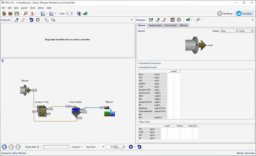
Figure 1‑24 – Simulation Environment
Notice that a standard unit process output tab for each unit in the layout (Influent, Aeration Tank, Final Clarifier, and Effluent) is automatically generated in the output section (Figure 1‑25). These are Quick Display summary tables, which will display output results after simulations are carried out.
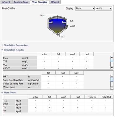
Figure 1‑25 - Quick Display Panels
You can quickly bring a desired Quick Display panel to the front by double-clicking on the unit process on the drawing board as an alternative to clicking on each individual process tab in the panel.
There are three subdivisions in the Quick Display panel:
1) Simulation Parameters. This sub-heading is used to display important information about the object’s operational parameters specified in Modelling Mode.
2) Simulation Results. This sub-heading provides a summary of the simulation results, highlighting some key characteristics of the influents, effluents and internal conditions
3) Mass Flows. This sub-heading provides a summary of the mass of TSS, COD, TN and TP that can be found in each stream entering and exiting an object.
Your model is now ready to run a simulation. The controls that you will need to run a simulation are located on the Simulation Toolbar found at the bottom of the screen.
![]()
Figure 1‑26 - Simulation Toolbar
|
|
24. Start the Simulation by pressing the Start button on the Simulation Toolbar. |
Pressing the start button will run a steady state simulation. Once the simulation is complete the tables in the output area will be populated with values.
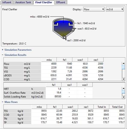
Figure 1‑27 – Clarifier Quick Display Simulation Results
25. Switch between the various Quick Display windows to view the simulation results for each unit process in the layout.
26. Save the Layout. Press the Save button on the main toolbar.
While steady state simulations provide the foundation of a model, the value comes from the ability to run dynamic simulations.
This tutorial covers the following topics:
1. Setting up graphics and interactive controllers
2. Running interactive simulations
When you have finished this tutorial, you will be able to run full-scale dynamic treatment process models. You will learn the procedures for creating time series graphics and interactive controls. These essentials provide a foundation on which other advanced features are built; therefore, it is important to understand the material in this tutorial first before going on to more complicated tasks.
GPS-X is an interactive simulation program, or simulator, which can run both pre-defined simulations and interactive sessions. We will now set up an interactive session that allows us to investigate the effects of changes in the influent flow rate on the plant effluent quality.
Our first task is to create a new Input Control. An input control is an interactive tool, which can be used to change the value of model variables during the course of a simulation run. You can create as many input controls as desired.
Here, we will create a single control for the plant influent flow so that this variable can be changed during a simulation.
1. Open the layout built in Tutorial 1 and save it as `tutorial-2’ using File > Save As...
2. Access the parameter by right-clicking on the influent object and select the Flow Data item from the Flow sub-menu as shown below.
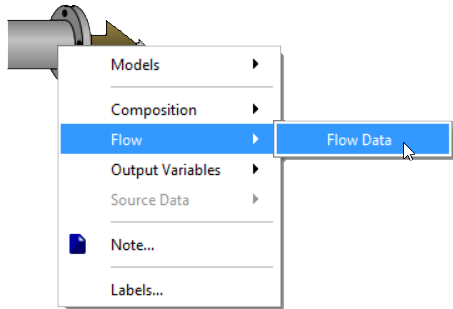
Figure 2‑1 - Accessing Flow Parameter
3. From the Flow Data entry form, drag the influent flow variable to the blank input control area above the layout, as shown below.
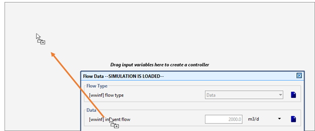
Figure 2‑2 – Dragging Variable to Control Tab
Note that a new tab (labeled “Input: 1”) has been created for the input control. Multiple controls can be placed on a single tab, or on as many tabs as required.
|
|
4. Edit the input control properties by clicking on the Input Control Properties… button on the Controls toolbar. An entry form window will be displayed. |
You can use this form to set minimum (Min), maximum (Max), and control increment (Delta) values (if applicable) for a particular variable.
Select 0 for Min and 12000 for Max. It is not necessary to enter a value in the Delta column, as we will use a slider-type control, which does not require a value for this attribute.
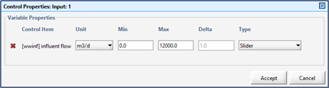
Figure 2‑3 – Control Properties Window
Note that you have the choice of a variety of controller types (under the Type heading). Make sure that Slideris selected for the influent flow item.
Remember to save your changes by pressing the Accept button.
5. Rename the control tab by double-clicking on the tab name “Input: 1”. Type “Flow Control” and pressEnter.
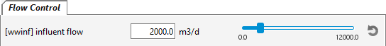
Figure 2‑4 – Finalized Input Control
An input control for the plant influent flow has now been created.
The tab shown in Figure 2‑4 contains a slider that allows you to change the influent flow from 0 to 12000 m3/d.
You can test the slider control by dragging the small slider knob. Note that the influent flow value will change to the value displayed on the control.
|
|
Before proceeding, use the Reset button at the far right of the slider to move the slider back to the default position of 2000 m 3/d (alternatively, you may enter the value into the control box with the keyboard). |
In addition to the summaries available on the Quick Display panels, you can create new custom-designed output graphs for numerous variables located in the Output Variables menu of each object that can be seen when right-clicking on an object.
These variables cover a wider range of model outputs and can be used to supplement the standard output in the Quick Displays.
|
|
6. Create a new, blank output tab by clicking on the New Graph Tab button on the Outputs toolbar. A new, blank output tab will be created. |
7. Create a graph of the influent flow by right-clicking on the influent object and select Output Variables > Flow as shown below.
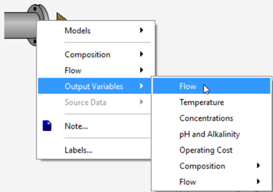
Figure 2‑5 - Accessing Output Variable Windows
8. From the Flow window, drag the influent flow variable to a blank area on the new tab that you created, as shown below. This will create an X-Y Graph with that variable on the y-axis. Select Accept or Cancel to close the Flow window.
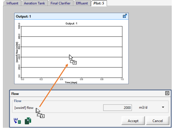
Figure 2‑6 – Dragging Variable to Create a Graph
9. Next, right click on the wastewater outfall unit and select Output Variables > Concentrations from the pop-up menu.
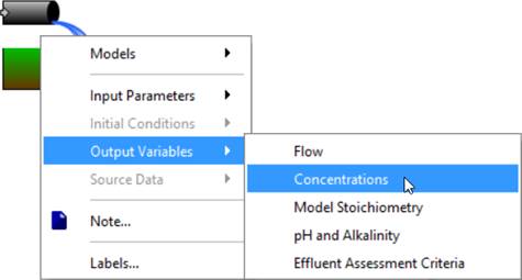
Figure 2‑7 - Accessing the Concentrations Menu from the Wastewater Outfall
Alternatively, if a Wastewater Outfall object were not used, this menu could be accessed by right clicking on the clarifier’s effluent overflow stream. When you place your cursor over the effluent overflow stream, the cursor will change from the default Microsoft cursor to the connecting arrow, that is seen in Figure 2‑8. Right click and select Output Variables > Concentrations from the pop-up menu. Note: Ensure the connection arrow is present because clicking on the center of the object will open a different menu than the connection point [2].
Figure 2‑8 - Connection Point Cursor Change
10. Drag the total suspended solids variable to the same graph as the influent flow. This will add another y-axis to the graph for this variable.
|
NOTE: There is a difference between data entry forms and output variable forms even though both have a similar appearance and may contain the same variable name entries. Data entry forms contain a field on the right-hand side for entering data. In output variable forms this field displays model results and cannot be edited. Variables dragged from a data entry form can be placed on input control tabs whereas variables dragged from an output variable form can be placed on graphs in the output field. |
|
|
11. Resize and arrange the graph by clicking on the Auto Arrange button on the Outputs toolbar. Your simulation environment should appear as shown below. |
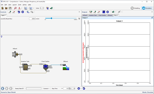
Figure 2‑9 - Simulation Environment with Output Graph
|
|
12. Access the output graph properties window by right-clicking on the output graph and selecting the Output Graph Properties… item from popup menu. Alternatively, you can press the settings button on the Output toolbar. |
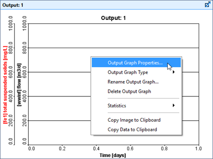
Figure 2‑10 – Accessing Output Graph Properties
The Output Graph Propertieswindow is used to specify plotting attributes including the min and max y-axis values, the color of the variable’s line and the units that the data will be displayed in.
The Autoscale feature can be used to allow the y-axis to automatically set an appropriate max value depending on the data being displayed (it will adjust during the simulation). By selecting this you will not have the option to adjust the values under the Variable Properties section of the Output Graph Properties window.
The Output Graph Type item is also available here. By default, the graph type is X-Y (time series) but this can be changed to several different options. For this tutorial, we will be leaving it as X-Y.
13. Enter a minimum and maximum value for each variable. Use 0 and 10,000 m3/d for flow, and 0 and 150 mg/L for total suspended solids.
|
|
NOTE: You must ‘unlock’ the max fields to be able to edit them individually otherwise the change in one field will be copied to the others. This is because quite often people will plot variables of similar characteristics on a graph and they’ll want the y-axis to have the same scale. |
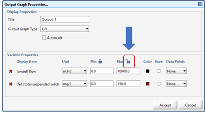
Figure 2‑11 – Output Properties showing Unlocked Max Field
Keeping the max fields unlocked, Accept the changes when you are finished.
14. Rename the output graph. This can be done in the properties window described above, but several of the properties can also be accessed from the popup menu by right-clicking on the graph. Do this and select Rename Output Graph…. Enter an appropriate title for the output graph and click OK.
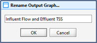
Figure 2‑12 – Rename Output Graph
You are now ready to run the model. All of the controls that you will need to run a dynamic simulation are located on the Simulation Toolbar at the bottom of the screen.
![]()
Figure 2‑13 – Simulation Toolbar
15. Specify a simulation duration time of 20 days by either entering the value directly into the Stop Time field or by repeatedly clicking on the up arrow adjacent to field to increment the value by 1 day for each click.
|
|
16. Start the simulation by clicking on the Start button. |
While the simulation is running you can now change the flow with the input control slider bar and assess the effect of changes in influent flow on the effluent suspended solids of the plant.
If the flow is high enough (say 7,000 m3/d) you will see a significant increase in the effluent suspended solids due to clarifier overload.
An example run is depicted in Figure 2‑14, where the flow was increased with the input control slider bar during the simulation run. Note that your output graph will look different than the one presented below depending on how you adjust the slider control during the simulation run.
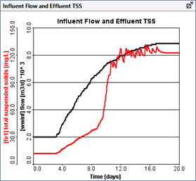
Figure 2‑14 – Example Run with Flow Increase
17. Run the simulation again, but this time, adjust the influent flow by dragging the influent flow slider away from 2,000 m3/d.
If the simulation proceeds too quickly, you can artificially slow down the simulation by inserting a delay. Add a delay by putting 0.5 (or any other number, the magnitude of the number dictates the degree of delay) into the Delay entry field using the Stop Time/Communication/Delay drop-down menu on the Simulation Toolbar.
|
NOTE: If the simulation time exceeds the stop time (Stop) the model will halt. At that time, you have two choices:
· Increase the length of the simulation by increasing the value of Stop and clicking Resume to continue the simulation. |
We will now take a more detailed look at our plant's performance by investigating the effect of increased flow on the secondary clarifier. We will first set-up an output graph displaying the solids profile inside the final clarifier. We will then simulate steady-state conditions with the design flow of 2,000 m3/d and investigate the change in the solids profile inside the final clarifier by running the model at a higher flow rate (i.e. simulating a storm condition).
To investigate the effect of increased flow on final effluent quality, you will first set up a graph to view the output of the solids profile inside the final clarifier.
18. Access the Concentrations of the clarifier by right-clicking on the object and selecting from the Output Variables > Concentrations.
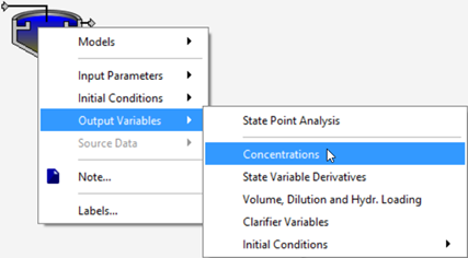
Figure 2‑15 - Accessing Concentrations
19. Drag the total suspended solids in layers (see Figure 2‑16) item to the blank area to the right of the existing output tabs. By dropping it there, a new tab is automatically created, and the desired graph is created on the new tab.
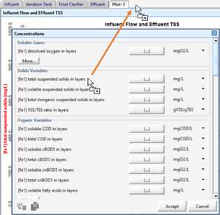
Figure 2‑16 - Dragging Variable to New Table
Since this variable is actually an array of values (denoted by the fact that it has an ellipsis (…) button next to it which can be used to access the individual values) then the graph that is created is by default a Bar Chart with the array elements along the x-axis.
20. Change the graph type. In this case, instead of the default vertical bar chart, we’d like to view the clarifier profile as a horizontal bar chart. This gives you a better intuitive feel of the different layers within the clarifier. The bar representing the bottom of the clarifier (index 10) will be at the bottom of the graph.
If you right-click on the output graph and select the Output Graph Typeitem, you will notice that the Bar Chart type has already been selected. Select the Bar Chart (Horizontal) type for this graph.
21. Change the axis max. Go into the graph properties and change the max value to 5000 mg/L.
22. Rename the graph. Right-click on the graph and select the Rename Output Graph… item from the drop-down menu and enter an appropriate title.
Note that you can also change the name of any tab by double-clicking on the tab name and entering a new one.
23. Resize the graph. Press the Auto Arrange button or drag the edge of the graph window to your desired size.
24. Select the Steady-State option andStart the simulation setting Stop to 10 days. Make sure that the influent flow is set to 2,000 m3/d on the input control. Below is a figure that shows a bar chart profiling the solids distribution inside the final clarifier.
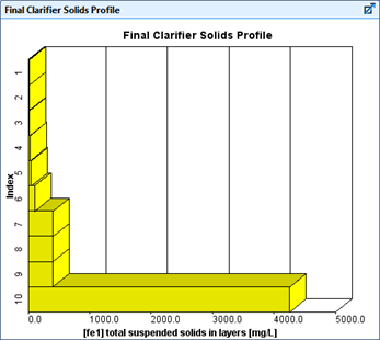
Figure 2‑17 – Clarifier Profile Graph
|
|
25. Increase the influent flowrate to a higher value (i.e. 5,000 m3/d) with the controller. Adjust Stop Timeto 20 days and Resume the simulation. |
The bar chart profiling the solids distribution inside the final clarifier will change to reflect the build-up of solids due to higher flows. You can adjust the max axis value to see the entire graph, if you’d like. The values will become greater than the existing scale.
26. Save the layout. Press the Save button on the main toolbar.
For this tutorial, consider a situation where the plant you developed in the first tutorial is expected to treat increased flow due, for example, to extra sewer connections. Assume that the plant has adequate aeration capacity but requires an extra clarifier.
GPS-X makes it easy to build models to help you examine changes in plant design and operation. This tutorial will show you how to use the layout editing tools such as Copyand Paste to make additions to the layout. Once the new model is built, the scenario features of GPS-X will be introduced. Using scenarios, you can set up specialized data sets for comparing the performance of the clarifiers in the event of uneven flow distribution under both steady state and dynamic conditions.
When you are finished with this tutorial, you will have
developed the ability to create and edit plant layouts and will
have developed a better understanding of static[3] data
input and output in GPS-X. You will be able to prepare
simulation scenarios to test different hypothetical situations and
be able to run the scenarios to test alternative plant designs or
examine operational changes.
1. Recreate the layout used in Tutorial 1 or open the layout that you previously created.
2. Save the layout under a different name (eg. tutorial-3).
3. Switch to Modelling Mode (if not already there) using the button on the top right-hand side of the screen.
4. Display the grid on the drawing board. Select View > Display Grid from the main menu.
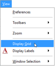
Figure 3‑1 - Selecting Display Grid
5. Display a larger drawing area. In order to expand on the layout, more space is required on the drawing board. Open the Locator window under View > Zoom > Locator and outline a larger working area. Alternatively, the mouse wheel can be used to scroll out and the desired work area can be highlighted and then zoomed in on by using the Zoom to selection/plant button. This will allow you to place more objects on the drawing board. More details regarding use of the Locator are presented in Tutorial 1.
6. Move the influent and plug-flow tank objects by clicking and dragging out a box around the influent and plug-flow objects. Then, with the mouse button pressed on one of the selected objects, drag the selected area to its new location on the drawing board (see Figure 3‑2).
7. Move the wastewater outfall object by clicking and dragging the object to the right.
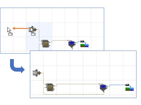
Figure 3‑2 – Moving Multiple Unit Processes
8. Copy the final clarifier. First, select the existing secondary clarifier located on the drawing board. The clarifier grid cell will show a light blue background.
|
|
Click on the Copy button and then select a destination cell by dragging out a small box inside the destination cell. The destination cell will show a light blue background. |
|
|
Next, click on the Paste button. This will paste a copy of the clarifier and all its attributes to the new location. |
Your layout should now look like Figure 3‑3.
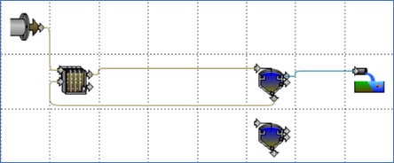
Figure 3‑3 - Copy/Pasted Clarifier
We will now complete the layout by adding the following:
· A two-way splitter to divide the mixed liquor from the aeration tank to the two clarifiers
· A two-way combiner to join the recycled sludge from the two clarifiers with the raw sewage as feed to the aeration tank.
· A two-way combiner to mix the effluent overflow from the two final clarifier tanks
9. Delete unneeded connections. You can delete a connection by right clicking on the connection and selecting Delete Connection.
Alternatively, you can delete the flow lines by placing the cursor at the initiation or terminal point of a flow line and dragging the flow line to an empty space on the drawing board. As soon as the mouse button is released you will be prompted to confirm the deletion of the flow line.
Delete the connection from the plug flow reactor to the final tank, the connection between the clarifier underflow and the plug flow reactor and finally the connection between the clarifier effluent and the wastewater outfall.
10. Add processes to the drawing board. From the Flow Combiners and Splitters group in the Process Table we will need one 2-Flow Splitter and two 2-Flow Combiners. Position the objects so that your layout now resembles Figure 3‑4.
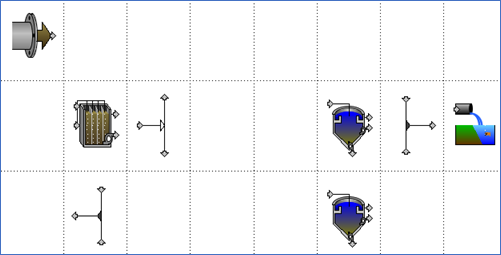
Figure 3‑4 - Add Splitter and Combiners
|
|
11. Flip the combiner below the Aeration Tank. To do this, select the combiner and press the Mirror button on the main toolbar. |
12. Connect all objects and label all units and streams. The last step of the plant expansion is to connect all the objects and label them appropriately as seen in Figure 3‑5 and described in Table 3‑1.
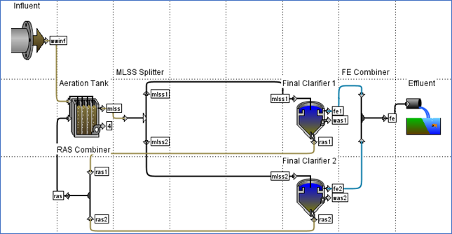
Figure 3‑5 - Processes and Streams Labelled Properly
|
NOTE: The colors of the flow lines each convey a specific meaning about the properties of the stream. Brown lines are used to represent the flows of wastewater. An example of this is your wastewater influent or the sludge leaving a clarifier Black lines are used to represent any streams where you are unable to tell what the outputs will be when the object is selected. An example of this is a combiner or splitter objects Blue lines are used to represent any flows of treated water. An example of this is the effluent stream leaving a clarifier overflow |
Table 3‑1 - Process and Stream Labels
|
Unit |
Label |
|
Wastewater Influent |
Label: Influent influent: wwinf |
|
Plug-Flow Tank |
Label: Aeration Tank overflow: mlss recycle: ras |
|
2-Flow Splitter |
Label: MLSS Splitter output#1: mlss1 output#2: mlss2 |
|
Circular Secondary Clarifier 1 |
Label: Final Clarifier 1 overflow: fe1 pump: was1 underflow: ras1 |
|
Circular Secondary Clarifier 2 |
Label: Final Clarifier 2 overflow: fe2 pump: was2 underflow: ras2 |
|
2-Flow Combiner for Recycled Sludge |
Label: RAS Combiner output: ras |
|
2-Flow Combiner for Final Effluent |
Label: FE Combiner output: fe |
|
Wastewater Outfall |
Label: Effluent |
13. Add a note to a process. Sometimes it is useful to make a note to remind yourself about certain details or reasons for changing something. These notes are just for your own reference and do not affect the simulation in any way.
Here, we will add a note to the Final Clarifier 2 unit. Right-click on it and choose Note… from the popup menu. A blank window will appear in which description of the unit can be typed. Click Accept to close the Note window.
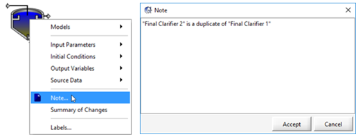
Figure 3‑6 – Add Note to a Process
14. Save the layout. Press the Save button on the main toolbar.
When organizing simulation runs it is useful to start with a base set of data, and then create one or more separate cases, which are modifications to the base data set. These cases are referred to as scenarios in GPS-X.
You can create any number of scenarios and in each scenario, you can specify the changes to the model parameter(s) which define that scenario. Those changes are saved so that they can be restored at any point in the future.
Creating and using scenarios is done in Simulation Mode.
In this section of the tutorial, we are going to use scenarios to investigate the effects of changing the following model parameters:
· Influent flow, to simulate the additional sewer connections
· Influent type, to simulate a dynamic fluctuation of the influent wastewater
15. Switch to Simulation Mode using the button at the top-right of the screen.
16. Create a new scenario by selecting Newfrom the Scenario menu on the Simulation Toolbar (at the bottom of the main window).
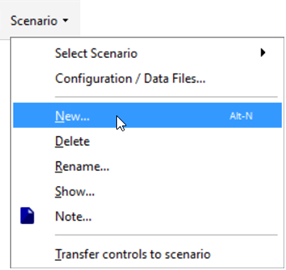
Figure 3‑7 - Create New Scenario
17. Type in a name for your new scenario (eg. “Expansion”) and Accept the form.
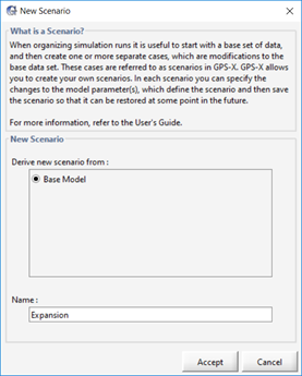
Figure 3‑8 – Name the Scenario
You will notice that the name of the active scenario is displayed under the Start button on the Simulation Toolbar.
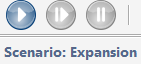
Figure 3‑9 - Scenario Name Display
|
NOTE: You can change the active scenario by selecting it from the Scenario > Select Scenario list. The “Default Scenario” is the base case where all of the model parameters are set to the values defined when the model was built. If you return to modelling mode and make changes to the Default Scenario Parameters, these changes will be applied to all scenarios where that parameter has not already been specified. |
18. Add some parameter changes to the scenario. In this case, we will change the influent flow type and rate.
While remaining in Simulation Mode, access Flow > Flow Data from influent objects process data menu (ie. right-click on the object).
Change the flow type to Sinusoidal and change the influent flow to 5000 m3/d.
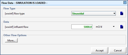
Figure 3‑10 - Changing Parameters in a Scenario
You will notice that changes made in a scenario are highlighted in green.
Accept the form.
19. If you do not already have an input controller (slider type) for the influent flow create one as described in the Creating Input Controls section of Tutorial 2. Set the minimum and maximum values to 0 and 12,000 m3/d respectively.
20. Verify the parameter changes made in the scenario. Any changes made in a given scenario from the base scenario can be viewed by selecting Show on the Scenario menu on the Simulation Toolbar.
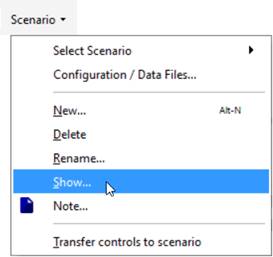
Figure 3‑11 - Show Changes Made to the Active Scenario
This window will show a summary of any variables that have been changed in the current scenario. The value that the variable was assigned when the model was built is shown in the grayed-out box. If any of the variables changed in this scenario appear on an input controller, an icon will appear next to the variable name to indicate the input controller.
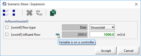
Figure 3‑12 - Summary of the Changes made in the Active Scenario.
|
|
Parameter changes in a given scenario can be directly edited in this menu by adjusting the setting of the box that is not grayed out. Additionally, any unwanted changes can be returned to their default value by checking the box next to the parameter name and pressing the Remove button in the toolbar. |
Accept the form.
21. Create an input control (slider type) for the split fraction (in the "MLSS Splitter"). Access this variable by going to Input Parameters > Splitter Setup. Set the minimum and maximum values to 0 and 1, respectively.
22. Create a horizontal bar chart for the solids profile in the new (copied) clarifier as described in the Analyzing the Plant section of Tutorial 2.
23. Create a X-Y graph for the effluent SS for each clarifier, and the combined effluent. In each case, the total suspended solids variable can be found in Output Variables > Concentrations of each object's outflow stream (ie. right-click on the connection point, not the process itself). Display all three concentrations on one graph and rename the graphs appropriately.
24. With the steady state box checked, run a 1-day dynamic simulation.
25. Change the split fraction to 0.3 using the interactive controller and increase the stop time to 2 days.
26. Resume the simulation using the Resume button (ie. don’t restart it) and let the simulation proceed until it stops.
27. Increase the flow to the plant to 8,500 m3/d, and increase the stop time to 3 days.
28. Resume the simulation.
A set of typical results are shown in Figure 3‑13. These graphs show the effect of the imbalanced flow split on final clarifier performance and combined final effluent SS.
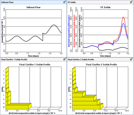
Figure 3‑13 - Typical Results
For this tutorial, consider that your supervisor needs you run the plant model on a monthly basis and present them with various reports and information regarding the plant performance, flow through the plant, energy usage, and operating cost.
GPS-X makes it simple to create customized tables, and reports, and export the data contained within them to a format that can be easily analyzed understood.
1. Open the layout built in Tutorial 3 and save it as `tutorial-4’ using File > Save As...
2. Switch into Simulation Mode if not already there.
In addition to the viewing model results and summaries on the Quick Display and various Graph outputs discussed in Tutorial 2 and Tutorial 3, you can also create custom-designed tables. These tables can be populated with a wide range of model outputs and present the data as a summary of stream or process variables across the layout.
|
|
3. Create a Table Tab. Press the New Table Tab button on the Outputs toolbar. This will open the Table Properties setup wizard. |
|
|
4. Populate the table. By default, all options are selected. We are only interested in a few streams and a few variables, so begin by pressing the Select None buttons at the top of each choice panel. This will deselect all options. |
Then make the following selections on the Stream Choice panel:
· Influent (wwinf) > wwinf
· Aeration Tank (mlss) > mlss
· Final Clarifier 1 (fe1) > fe1
· Final Clarifier 2 (fe2) > fe2
· FE Combiner (fe) > fe
On the Variable Choice panel, select the following:
· Solids > TSS & VSS
· Organic Variables > COD
· Nitrogen Variables > Ammonia Nitrogen & Nitrate & Nitrite
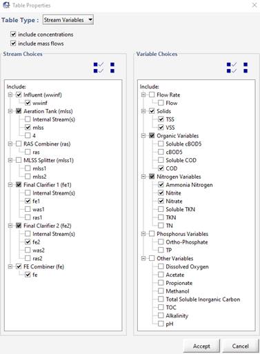
Figure 4‑1 – Table Display Setup Wizard
5. Press Accept to create the table.
6. Run a Steady State simulation of the “Default Scenario” located in the Simulation toolbar under Scenario > Select Scenario and observe the new table tab. From the table we can observe the reduction in the TSS and COD concentrations across both secondary clarifiers (mlss and fe1/fe2 streams); and the nitrification occurring across the aeration tank (wwinf and mlss streams).
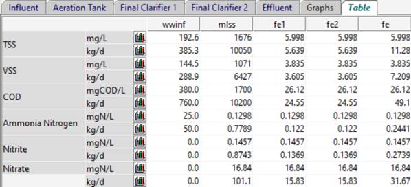
Figure 4‑2 - New Table Tab Output
|
|
7. Export the table. Save a copy of the data in this table by selecting the table tab (if it’s not already shown) and press the Export button on the Outputs toolbar. This will open a drop-down menu with the options to export as a Microsoft Word or Microsoft Excel file. Selecting either option will open a file browser where you can select an appropriate location and name for the file. |
|
|
8. View the data as a Bar Chart. If you would like to visualize the data in a particular row, click the bar chart icon next to the unit. This will create a new tab with the appropriate bar chart. |
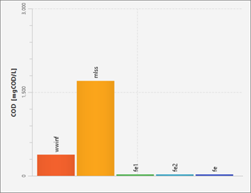
Figure 4‑3 – Bar Charts from Table Display for COD
9. Save the layout.
|
|
10. After running a simulation, options in GPS-X, it will unlock to analyze the results of the simulation. On the Outputs toolbar, the Additional Output Displays option will become enabled. |
11. Selecting the Additional Output Displays option will open a drop down menu with various useful tools for visualizing the outputs of the simulation. We will now explore each option available in this menu.
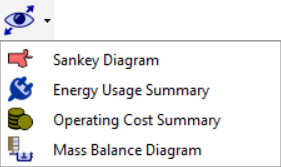
Figure 4‑4 - Additional Output Displays Menu
GPS-X can create a Sankey diagram of five variables (Flow, TSS, COD, TN, and TP). Sankey diagrams are flow diagrams that display variable quantities in terms of arrow width. This allows users to look at the plant's performance visually and display the results effectively.
|
|
12. Open the Sankey Diagram window. Once a simulation run has been completed, select the Sankey Diagram option from the Additional Output Diagrams drop down menu. This will open the Sankey Diagram window. |
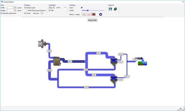
Figure 4‑5 - Sankey Diagram Example
Figure 4‑5 shows a Sankey Diagram of the system flow rates. The diagram displays the Sankey graph and the values for each stream.
Notice that a stream with a higher flow rate displays a wider arrow. In this example, the flows out of the clarifiers illustrate this. The effluent stream (940 m3/d) has a much bigger arrow than the tiny arrow exiting the pumped flow (60 m3/d).
You can change settings and output variables using the Display, Variable, and Sankey features on top of the Sankey diagram window.
The Sankey diagram can be exported using the Export features.
The values represented visually by the thickness and color of the lines in a Sankey Diagram can also be represented numerically in a Mass Balance Diagram.
|
|
13. Open the Mass Balance window. Once a simulation run has been completed, select the Mass Balance Diagram option from the Additional Output Diagrams drop down menu. This will open the Mass Balance Diagram Wizard menu |
This menu will allow you to select what information you would like to be displayed on the diagram. The Columns options can be used toggle the display of concentration and/or mass flow rates while the Rows options can be used to select the variables of interest.
Press Next.
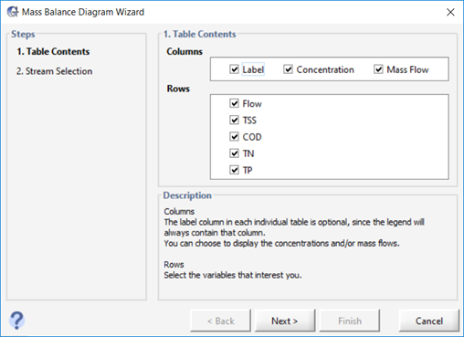
Figure 4‑6 - Mass Balance Setup Wizard Table Contents
|
|
14. Select the Streams. The Mass Balance Wizard will initially select all of the streams on the drawing board, but we are only interested in a few of the streams. Press the Select None button to deselect all options. |
Select the following options from the menu:
· Influent (wwinf) > wwinf
· Aeration Tank (mlss) > mlss
· Final Clarifier 1 (fe1) > fe1
· Final Clarifier 2 (fe2) > fe2
· FE Combiner (fe) > fe
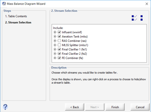
Figure 4‑7 - Mass Balance Setup Wizard Stream Selection
15. Press Finish to confirm the streams you would like to be shown in the diagram.
16. Auto Arrange. After selecting finish, you will be prompted to auto arrange the table locations. By selecting this option, GPS-X will align all of the tables along the top and bottom of the diagram close to the stream it is creating a table for. Choosing not to auto arrange the tables will use a previous table layout if available. In this case, it will produce the same layout as auto arrange.
After accepting auto arrange, the Mass Balance Diagram will open. You can click and drag the tables anywhere you would like in the diagram window. Figure 4‑8 shows a Mass Balance Diagram of the system after the user has manually arranged the tables. The diagram displays the mass and concentration flow rates of the variables in each stream of interest.
The Mass Balance Diagram can be exported using the Export features.
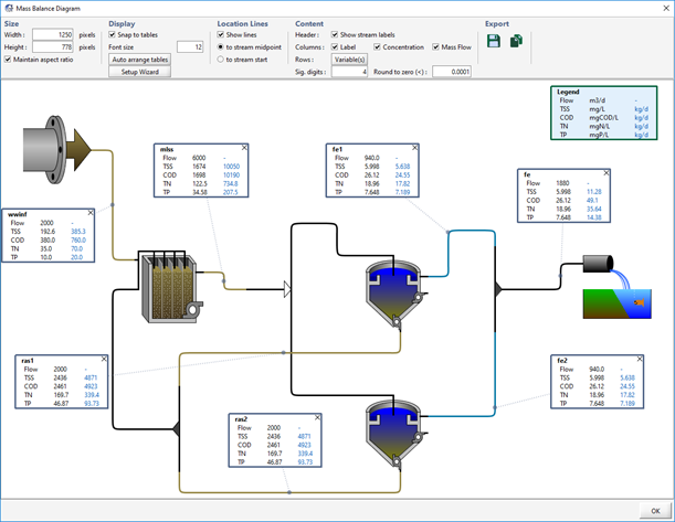
Figure 4‑8 - Mass Balance Diagram Example
After a simulation has been run, you can choose to view a plant schematic output summary of either the Energy Usage or Operating Costs. First let’s explore the Energy Usage Summary.
|
|
17. Open the Energy Usage Summary window. Once a simulation run has been completed, select the Energy Usage Summary option from the Additional Output Diagrams drop down menu. This will display the Energy Usage summary window |
In the window, an image of the layout is shown with ‘hot spots’ around the unit processes that represent the value of the variable that is being displayed. The intensity of the color of the ‘hot spot’ increases as the value gets larger.
By selecting a different type of power usage from the “Variable” pull-down menu, you can view a summary of the different types of power used in the plant (aeration, pumping, mixing, etc.).
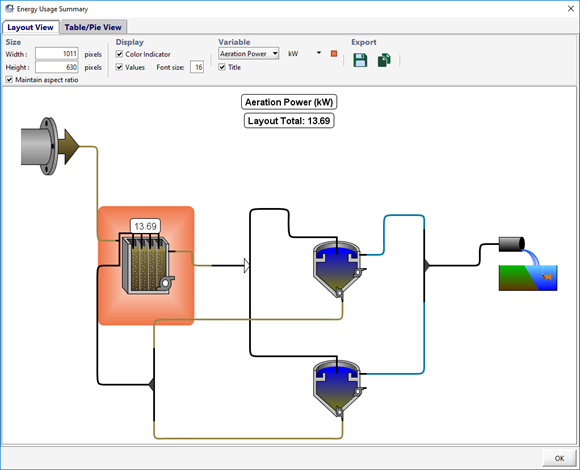
Figure 4‑9 - Energy Usage Summary Window
18. Click on the Aeration Tank. This will take you to the “Table/Pie View” and select the row that corresponds to the aeration tank. Changing the selected row/column will change the pie chart to display the appropriate data.
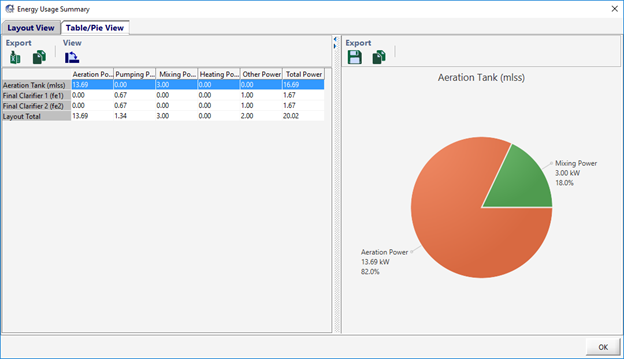
Figure 4‑10 - Table/Pie View of Aeration Tank
19. Press OK to close the window.
We will now explore the Operating Cost Summary.
|
|
20. Open the Operating Cost Summary window. Once a simulation run has been completed, select the Operating Cost Summary option from the Additional Output Diagrams drop down menu. Selecting it will display the Operating Cost summary window. |
You will notice that this window is arranged in a similar manner to that of the Energy Cost Summary window. An image of the layout is shown with ‘hot spots’ around the unit processes that represent the value of the variable that is being displayed. The intensity of the color of the ‘hot spot’ increases as the value gets larger.
By selecting a different type of costing from the “Variable” pull-down menu, you can view a summary of the different types of operating cost that exist in a plant (aeration, chemical dosing, sludge disposal).

Figure 4‑11 - Energy Cost Summary Window
21. Click on the Aeration Tank. This will take you to the “Table/Pie View” and select the row that corresponds to the aeration tank. Changing the selected row/column will change the pie chart to display the appropriate data.
You may wish to create a report with a list of all the parameter values, as well as the model results for a particular simulation. The reports are generated in Microsoft Excel or Microsoft Word format.
|
|
22. Click on the Report button in the main toolbar (NOT the button with a similar icon on the Output toolbar. That one will just export the selected output display). |
This will open a window where you can create a Standard Word Report, or create a Standard or Custom Spreadsheet Report.
23. Click on the Report button in the main toolbar (NOT the button with a similar icon on the Output toolbar. That one will just export the selected output display).
This will open a window where you can create a Standard Word Report, or create a Standard or Custom Spreadsheet Report.
24. Select Standard Spreadsheet Report. The Options button beside it allows you include/exclude certain data from the report.
25. Press the Generate button. A file browser will be displayed where you can choose an appropriate directory and file name.
26. View the Report. After it’s created, you will be asked if you want to open the file. Click Yes, and the report will be opened in Excel. Browse through the various worksheets to see the model layout, details of each object, and output graph data
You have some historical data related to the influent wastewater for your plant and it does not resemble the default data presented in the GPS-X influent object forms. Unfortunately, a full characterization of your influent wastewater has not been performed. Nevertheless, you need to estimate the influent wastewater characterization so that the model can be used with an influent that approximates your influent data.
In this tutorial, you will investigate the influent models, the impact of the local biological model on the influent calculations and the use of Influent Advisor as a tool to help characterize influent data.
The following historical data have been gathered at your plant and represent average values for your influent.
Table 5‑1 – Average Historical Data
|
Measured Parameter |
Value |
Units |
|
total COD |
365 |
gCOD/m3 |
|
ammonia nitrogen |
26 |
gN/m3 |
|
total TKN |
36 |
gN/m3 |
|
total carbonaceous BOD5 |
190 |
gO2/m3 |
|
filtered COD |
68 |
gCOD/m3 |
|
total suspended solids |
210 |
g/m3 |
|
volatile suspended solids |
168 |
g/m3 |
|
filtered TKN |
31 |
gN/m3 |
|
|
1. Create a New Layout. Press the New button on the main toolbar. |
2. Select a library. In this tutorial, we will be using the Comprehensive – Carbon, Nitrogen, Phosphorus, pH (mantis2lib) library. If it isn’t already selected, choose it from the Library menu.
3. Place an influent object on the drawing board. From the Influent group in the Process Table, drag a Wastewater Influent object on the drawing board.
4. Save the layoutas `tutorial-5’.
5. Switch to Simulation Mode. We will be using a scenario to demonstrate the changes for this case study.
6. Create a new scenario named Influent. This process is described in Tutorial 3 in the Using Scenarios section.
7. Open the Influent Advisor tool. To do this, right-click on the influent object and select Composition > Influent Characterization.
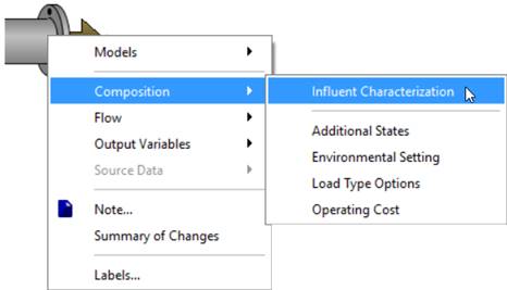
Figure 5‑1 - Accessing Influent Advisor Tool
8. Adjust values under “User Inputs”. You’ll notice that under the “User Inputs” section of the Influent Advisor tool are various values that you can change. From our list of data in Table 5‑1, only the first three values are immediately accessible.
Enter the values for total COD, total TKN and ammonia nitrogen.
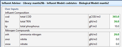
Figure 5‑2 – Adjusted Values
The entries are shown in green, indicating that these changes are part of the Influent scenario you created earlier.
9. Check the remaining data in the table against their corresponding values in the Influent Advisor. You will find the remaining variables in the right-most column (Composite Variables).
The values reflect the new COD, TKN and ammonia input, but use the default influent fractionation.
Note that the plant data differs from the calculated values displayed in the Influent Advisor tool.
Table 5‑2 - Plant Data vs Calculated Data
|
Parameter |
Plant Value |
Displayed Value |
Units |
|
total COD |
365 |
- |
gCOD/m3 |
|
ammonia nitrogen |
26 |
- |
gN/m3 |
|
total TKN |
36 |
- |
gN/m3 |
|
total carbonaceous BOD5 |
190 |
188.2 |
gO2/m3 |
|
filtered COD |
68 |
125.2 |
gCOD/m3 |
|
total suspended solids |
210 |
185.3 |
g/m3 |
|
volatile suspended solids |
168 |
139.0 |
g/m3 |
|
filtered TKN |
31 |
28.9 |
gN/m3 |
Clearly, the influent model calculations are inconsistent with the data for your plant indicating that one or more of the default settings (i.e. composition data or stoichiometric fraction) are inconsistent with your wastewater.
In the next section, we will investigate the steps required to reconcile these discrepancies.
The Influent Advisor tool has been designed to make the characterization of the influent waste stream as straightforward as possible. It would be possible to run a series of simulations (while adjusting influent parameters on sliders and observing plotted outputs) to find the correct settings, however this method would require setting up input controllers and output tables/graphs and could be potentially time-consuming.
The Influent Advisor tool shows all input and output in an interactive way, allowing users to determine which inputs affect each output, and to trace all dependencies. The window contains three columns:
· User Inputs
· State Variables
· Composite Variables
We will now browse the various calculations and variables that make up our desired data.
10. Find the VSS variable in the Composite Variables column and click on the value. The VSS row will be highlighted and if you scroll up and down the page, you will also notice that several other rows have been highlighted in a lighter blue color. These are the variables that are used to calculate the VSS value.
Right at the bottom of the tool (scroll down), the actual formula is displayed (see Figure 5‑4). This formula corresponds to the formula used in GPS-X to calculate the value clicked on, in this case vss.
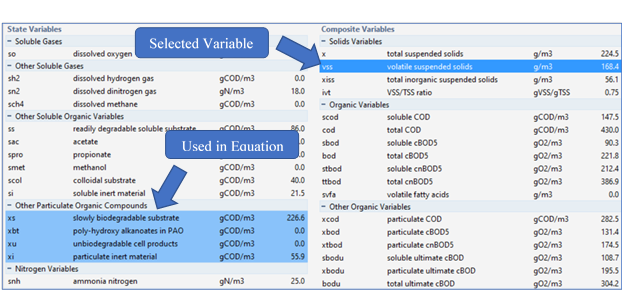
Figure 5‑3 – Influent Advisor showing Variable Relationships

Figure 5‑4 – Equation for VSS
Let’s proceed to adjust the influent parameters (fractions and/or concentrations) to reconcile the model predictions with the measured values.
11. Note that the particulate VSS to TSS ratio is used in the calculation of TSS. Select total suspended solids (x) from the Composite Variables table. This is one of several important relationships that can be calculated from the existing data. For instance:
VSS:TSS ratio (ivt) = 168/210 = 0.8
12. Enter this value into the User Inputs column under the Influent Fractions sub‑heading. Note that doing this seemingly results in values further away from what you are looking for. Further changes will be required.
13. Click on VSS to display the calculation formula. By continuing to click on the cells in the formula, you should be able to determine that vss is a function of the Particulate Organic Compounds, such as xi (particulate inert material), xu (unbiodegradable cell products), and xs (slowly biodegradable substrate). The VSS is lower than our target, meaning that we must distribute more of the influent COD to the particulate forms (and less to the soluble forms).
14. Adjust the stoichiometric ratios in the Organic Fractions sub-heading to increase the particulate COD concentrations. Try the following changes:
· set soluble inert fraction of total COD to 0.02,
· set readily biodegradable fraction of total COD to 0.15, and
· set colloidal fraction of slowly biodegradable COD to 0.05.
These changes force more of the COD into the xs (slowly biodegradable substrate) state variable, which therefore increases VSS and TSS.
15. Lastly, adjust the soluble TKN (stkn) value under the Composite Variables > Nitrogen Concentrations Headings. Click on the equation to determine the appropriate input parameter(s) to adjust and make the necessary change(s). You may find that adjusting the nitrogen variables causes the TSS to change. Make further adjustments to the influent COD fractions to bring the TSS back to the target.
|
NOTE: In reality, you will characterize your influent and adjust these unknown parameters based on the model behavior and how that model behavior relates to what has been observed or measured at the plant. Each wastewater is different, and each will require some adjustment of these parameters to get a characterization that results in model behavior that is consistent with your plant behavior. |
An example of one possible solution to the influent characterization is shown in Figure 5‑5 and Table 5‑3 below.
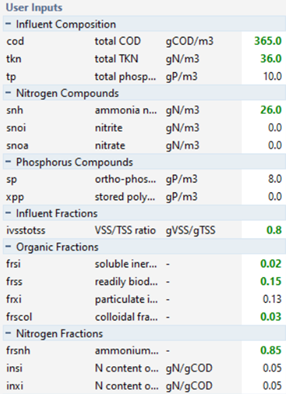
Figure 5‑5 - User
Inputs
Table 5‑3 - Plant Data vs Entered Data with Calculated Results
|
Parameter |
Plant Value |
Entered Value |
Shown Value |
Units |
|
total COD |
365 |
365 |
- |
gCOD/m3 |
|
ammonia nitrogen |
26 |
26 |
- |
gN/m3 |
|
total TKN |
36 |
36 |
- |
gN/m3 |
|
total carbonaceous BOD5 |
190 |
- |
188.5 |
gO2/m3 |
|
filtered COD |
68 |
- |
69.7 |
gCOD/m3 |
|
total suspended solids |
210 |
- |
209.7 |
g/m3 |
|
volatile suspended solids |
168 |
- |
167.7 |
g/m3 |
|
filtered TKN |
31 |
- |
30.6 |
gN/m3 |
|
VSS/TSS ratio |
- |
0.8 |
- |
gVSS/gTSS |
|
soluble inert fraction of total COD |
- |
0.02 |
- |
- |
|
readily biodegradable fraction of total COD |
- |
0.15 |
- |
- |
|
colloidal fraction of slowly biodegradable COD |
- |
0.03 |
- |
- |
|
ammonium fraction of soluble TKN |
- |
0.85 |
- |
- |
Strictly as an exercise to demonstrate a point, you will now change the influent characterization so that a warning message is generated due to an improperly characterized influent.
16. Change the total TKN value (tkn) to 15 mgN/L and hit ‘Enter’.
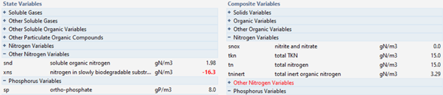
Figure 5‑6 - An Example of an Error in the Influent Advisor
You will notice that some state and composite variables have been highlighted in red. If a value in a collapsed menu is highlighted, that menu’s title will be highlighted red. This indicates a negative value. These negative values can sometimes be the result of unusual or poor characterization data. Negative influent concentrations can cause mass balance errors and convergence problems, so these values must be addressed before proceeding with a simulation.
Note that if you attempt to Accept an improperly characterized influent, a pop up will be generated to warn you that the input values have resulted in negative state or composite variables and you will be unable to accept the characterization until this value has be addressed.
The Dynamic Data Validation tool is used to validate a dynamic input data set prior to using it to run a dynamic simulation. The tool will take the input data and preform influent characterization calculations at each time step in the data set, identifying any negative values.
|
|
17. Access the Dynamic Data Validation Tool. The Dynamic Data Validation tool can be found in the toolbar at the bottom of the Influent Advisor tool window. |
![]()
Figure 5‑7 - Influent Advisor Toolbar
18. The Dynamic Data Validation Tool window will open and you will be required to add a pathway to both an input and an output data file.
There are two methods in which you can prepare the input file:
A. Manually prepare the spreadsheet outside of GPS-X and adding it directly to the Dynamic Data Validation Tool using the Browse button (Best used for multiple variables). Refer to Tutorial 6 for instructions on manually preparing spreadsheets.
B. Use the Create Template tool in GPS-X to automatically prepare the file (best for single variables).
This tutorial will focus on Method B.
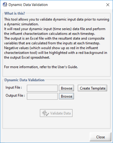
Figure 5‑8 - Dynamic Data Validation Window
19. Press the Create Template button.
20. Select the Parameters. GPS-X will prompt you to select the parameters you would like to include in the dynamic data validation.
Select the following parameters:
· cod / total COD
· tkn / total TKN
· snh / Ammonia Nitrogen
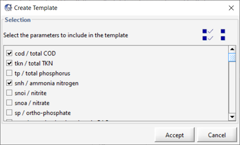
Figure 5‑9 - Dynamic Data Validation Parameter Selection
21. Save the file by pressing Accept. You will be prompted to save the Excel spreadsheet in the active directory using the same name as the layout. Press Save.
22. Open the file. GPS-X will prompt you to open the newly created spreadsheet. Press Yes.
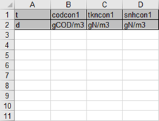
Figure 5‑10 - Excel Spreadsheet Generated by GPS-X
23. Enter the data found in Table 5‑4 into the Input File. The bold red values in the table correspond to the poorly characterized values that will cause influent advisor to calculate a negative value.
Table 5‑4 - Data for Dynamic Data Validation
|
t |
codcon1 |
tkncod1 |
snhcod1 |
|
d |
gCOD/m3 |
gN/m3 |
gN/m3 |
|
0 |
370 |
36 |
25 |
|
1 |
375 |
36 |
40 |
|
2 |
374 |
37 |
25 |
|
3 |
376 |
38 |
26 |
|
4 |
373 |
40 |
29 |
|
5 |
378 |
42 |
28 |
|
6 |
380 |
15 |
28 |
24. Save the changes made to the Excel Spreadsheet.
25. Create an Output File. Press the Browse button next to the Output File entry field. You will be prompted to create an output file in the current working directory. Press Save.
26. Press Validate Data.
27. The results of the data validation will be recorded in the output file. After validating the data, GPS-X will prompt you to open the output file. Press Yes.
28. The Output File of the Dynamic Data Validation can be seen in Figure 5‑11.
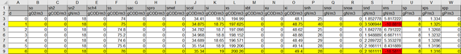
Figure 5‑11 - Output of the Dynamic Data Validation
Notice that row(s) 4 and 9 are highlighted yellow and contain cells that have been highlighted with a red background. The yellow rows indicate that the influent conditions used at this time step results in a negative value being calculated in the influent characterization. The red cells indicate the negative values calculated in the influent characterization
You are interested in testing your plant under more dynamic or stressful conditions such as a storm. Unfortunately, you do not have access to real storm flow data. Therefore, you will generate a simulated storm loading to your plant and then input this data as a driving function for the model. You will investigate the effect of step feed during the storm.
Interactive controllers provide an easy-to-use method for exploring the dynamic response of the model. However, in most modeling projects, it is desirable if not essential to input real forcing functions to examine how the model behaves under real conditions. The forcing functions can be flows or influent concentrations, or any other model parameter, but are always in the form of time dynamic data; that is, variable values over time. A typical set of time dynamic data would be the influent flow rate to the plant over a period of time. GPS-X facilitates the input of this data so that the model will be tested against real conditions.
This chapter covers an important and useful feature of GPS-X:
· Using a data file as an input to control simulations
1. Open the layout built in Tutorial 2 and save it as `tutorial-6’ using File > Save As...
2. Switch to Simulation Mode.
3. Create Input Controllers. More information regarding input controllers is presented in Tutorial 2. Right-click on the influent and select Composition > Influent Characterization to bring up the Influent Advisor tool.
The Influent Advisor will take up most, if not all, of the room on the main window. Click the little right arrow (see Figure 6‑1) between the “User Inputs” column and “State Variables” column to shrink the window and hide everything except the “User Inputs” column.
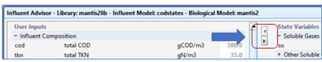
Figure 6‑1 – Shrink Influent Advisor
Now that you have room, drag total COD, total TKN and ammonia nitrogen to the controls section to create interactive sliders.
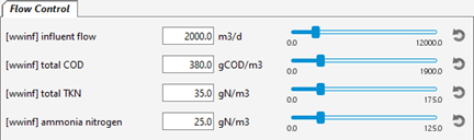
Figure 6‑2 – New Input Controllers
The next step is setting up the data in files to be read by GPS-X during a simulation. There are two different ways that data files can be prepared for the file input controllers:
A. Manually preparing spreadsheets outside of GPS-X (best used for preparing data for multiple variables) and adding the data file to the layout in Scenario > Configuration.
or
B. Using the Data File… tool in the GPS-X to automatically prepare the file (best used for preparing data for a single variable).
This tutorial will use both methods to illustrate their use.
|
|
4. To open the Data File organizer window, press the Data File button on the main toolbar in GPS-X. |
4. Press the New button to open the Data File Creation Wizard.
5. Ensure Input Variable is selected in the ‘Input or Output’ pane of the Data File Creation Wizard. Press Next.
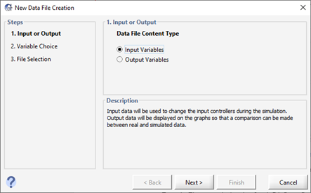
Figure 6‑3 – Data File Creation Wizard
6. Select the Variables. All of the input variables that are currently used to make an input controller will be available to add to a data file.
From the Flow control tab, select [wwinf] influent flow, [wwinf] total COD, [wwinf] total TKN and [wwinf] ammonia nitrogen. Press Next.
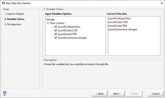
Figure 6‑4 - Input Variable Selection
7. Save the File. By default, GPS-X will save the excel sheet in the active directory with the same name as the layout. Press Finish.
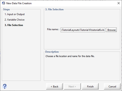
Figure 6‑5 - Save New Data File
8. Open the file. You will be prompted to open the new file after saving it. Press Yes.
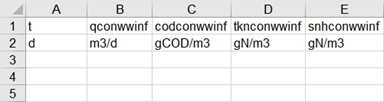
Figure 6‑6 - Input Data File Generated by GPS-X
We have created a version of this data file that has already been populated with data to use for this portion of the tutorial. Locate and open the tutorial-6-example-data.xls spreadsheet file in the following subdirectory of the GPS-X installation:
\layouts\08tutorials\
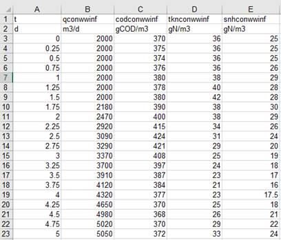
Figure 6‑7 – Contents of “tutorial-4-example-data.xls”
We will use the data found in this file as our dynamic dataset. It is a typical set of influent input data that you might use to simulate a change in influent loading over time.
The first column is labeled “t” for time, and is in the units of days “d.”
The remaining columns contain data for each of the parameters being read from the file. The names at the head of each column are the “cryptic variable name” (which is the internal “short form” variable name within GPS-X calculations) for each variable. These names are specific to the layout you have created and are different for each variable and object within the layout.
9. Verify that the cryptic names in the data file are the same as the variables for the input controllers. The simplest way to do this is to look at the tooltip that pops up when you hover the mouse cursor over the controller’s label as shown in Figure 6‑8.
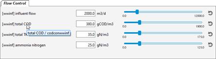
Figure 6‑8 – Viewing the Cryptic Name via Tooltip
The cryptic variable names for the four variables used in this tutorial are:
qconwwinf – influent flow
codconwwinf – total COD
tknconwwinf – total TKN
snhconwwinf – ammonia nitrogen
If the variables you are interested in are not currently on an input controller, you can quickly find the cryptic variable name by using the GPS-X find functionality. You can access the find function by going to Edit > Findon the main tool bar or using CTRL-F.
This will open the Find pop-up window. In the ‘Find Input/Output Variable’ pane of the find window there is an input box with a toggle for Keyword and Cryptic beneath it.
If you need to find a cryptic variable name and you know part of its plain English variable name, type it in the entry field and select, for example ‘total COD’. Ensure the keyword option is selected and press find. This will find and display every variable in the model that contains the keywords ‘total COD’. The matching variables will be grouped by the object they are associated with. The stream associated with the variable will be given in front of the variable name.
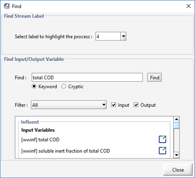
Figure 6‑9 - Finding all Instances of total COD in the Model
If a variable is related to a stream number/name that you do not recognize, use the ‘Select label to highlight the process’ drop down menu in the ‘Find Stream Label’ pane to select the stream. This will highlight the object that the stream initiates from on the layout. For example, selecting the stream ‘mlss’ from the drop down menu will highlight the Aeration tank.
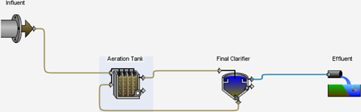
Figure 6‑10 - Using the Find Stream Label Functionality to Identify where the mlss Stream Originates
|
|
After identifying the variable of interest under the influent > Input Variables headings you can click on the Go to location button to the right of the variable to be taken to the window where this variable is defined. Hovering the cursor over the variable name will cause a tooltip containing the cryptic variable name to appear. |
Alternatively, if you are given a cryptic variable name by a GPS-X output, the corresponding plain English variable name can be identified using the find functionality. For example, after opening the find window, select the cryptic option and enter the cryptic variable name codconwwinf in the find field. Pressing the Find button will present you with input and output variable which have a cryptic name containing codconwwinf.
|
Note that “wwinf” in the cryptic variable name above comes from the label for the influent stream (eg. if you had labeled the influent stream as “1”, the cryptic name for influent flow will show up as “qcon1”). |
10. Access the Configuration window. Click on the Scenario menu on the Simulation Toolbar and select Scenario > Configuration/Data Files… > Data Files.
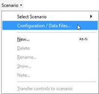
Figure 6‑11 - Accessing Scenario > Configuration/ Data Files…
Access the list of current data files. The configuration window will show all the scenarios available (in this case it should just be the Base Model). Data files can be added to a specific scenario if desired by selecting it before pressing the Data Files button. Make sure Base Model is selected and press the Data Files button.
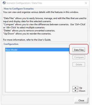
Figure 6‑12 – Scenario Configuration showing Data Files button
11. Add the data file. The Data Files window shows all of the files that this scenario is currently using. At this point, there won’t be any files displayed. To add the Excel file prepared above, press the Add button and browse to the appropriate location and select the tutorial-6-example-data.xls file.
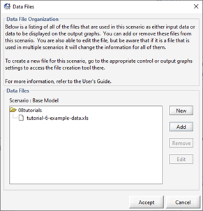
Figure 6‑13 – Adding File to Scenario
12. Accept the changes and close the Scenario Configuration window. Notice that the interactive slider for the inputs have automatically changed to file input controls that cannot be directly edited. The values are now being read in from the file.
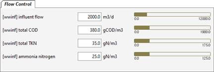
Figure 6‑14 – Controllers Changed to File Input
13. Run a 5-day simulation with Steady-State click ON. As the simulation proceeds, the values of the influent flow and concentration will change in the input controller. The model responds dynamically to the changing input, as shown in the increasing effluent solids.
The above methodology is useful for simulations where data for many parameters are being read in simultaneously, and it is easy to assemble that data externally in a spreadsheet.
There is another option that is useful for simple simulations where just one or two parameters are being read from a file, and you want to input those values directly into GPS-X. For this situation, you can use the Data File Tool.
14. Create another Input Controller. Right-click on an open spot in the layout background, and select System > Input Parameters > Physical Environment Settings. Drag liquid temperature to a new input tab (i.e. drop it in a blank area beside the current tab’s label). This will create a new slider controller on a new tab.
15. Rename the tab to “Temperature”.
16. Access the Data File tool for this input. Right-click on controller’s label (liquid temperature) and select the Data File… option. A new window will be displayed.
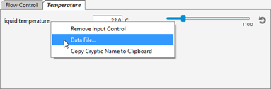
Figure 6‑15 – Accessing Data File Tool
17. Enter the data from Table 6‑1. Select a cell in the table and type the value. Using the tab key, you can move to the next cell.
Table 6‑1 - Data for Liquid Temperature Controller
|
t [d] |
temp [C] |
|
1 |
17 |
|
2 |
18 |
|
3 |
20 |
|
4 |
22 |
|
5 |
24 |
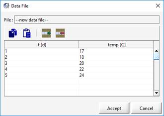
Figure 6‑16 – Data File Tool with Values
18. Save the data by pressing Accept. You will be prompted to save the file. The default location is the same directory as the layout file and the default name is the layout’s name with the cryptic name of the variable concatenated to it. These defaults are usually appropriate, so click Save to save the file.
Notice that the interactive slider for the liquid temperature input has automatically changed into a file input control bar and is no longer able to be manually adjusted.
19. Run a 5-day simulation with Steady-State clicked ON. As the model is simulated, the value of influent flow, concentrations and temperature will change in the input controller.
The previous section described the method for importing input data to the simulation file. In this section, the method for importing and displaying the measured output data onto a graph alongside simulated results will be introduced. This is convenient for comparing the measured value from a plant with the simulated results given in GPS-X. It also makes it easier to calibrate and optimize the process (see Tutorial 10 for details regarding optimization).
20. Create a spreadsheet file with example measured data. The table below is an example of the observed total suspended solids data for the final effluent from our example plant. Create a data file with this information and save it in the same directory as the layout file.
Table 6‑2 – Measured Data
|
t |
xfe1 |
|
d |
mg/L |
|
0 |
12 |
|
1 |
11.8 |
|
2 |
13.7 |
|
3 |
18 |
|
4 |
25 |
|
5 |
28 |
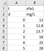
Figure 6‑17 - Excel Spreadsheet with Values
The cryptic variable name for the total suspended solids in the final effluent (xfe1) can be found by right-clicking on the output graph created in Tutorial 2 and selecting Output Graph Properties… from the drop-down menu. Hold the mouse cursor over the variable label and a tooltip will appear with the label/cryptic information as shown in Figure 6‑18. This should correspond to the name on the first row of the spreadsheet file.
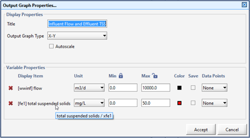
Figure 6‑18 – Tooltip showing Cryptic Variable Name
21. Add the data file. Following the same procedure as the last section where we added an input data file to the layout, access Scenario > Configuration/Data Files… > Data Files and add this new file to the layout.
22. Run a 5-day simulation with Steady-State clicked ON. The data points from the measured data is shown as diamond-shaped points on the graph, as shown in Figure 6‑19.
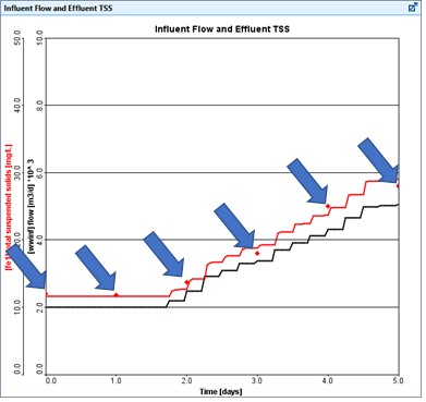
Figure 6‑19 – Graph showing Measured Data Points
A statistical analysis can then be conducted within GPS-X to test the model’s ability to reproduce the observed data. Statistical Analysis can only be preformed on X-Y timeseries output plots that have data points displayed on the plot.
23. Run a 5 Day Simulation.
24. Open the Statistics Menu. Right click anywhere on the graph and select the statistics > [fe1] total suspended solids option.
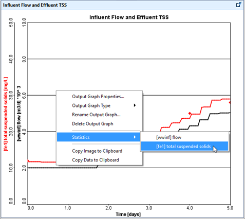
Figure 6‑20 – Accessing the Statistics Menu for Total Suspended Solids
25. Select the Statistical Analysis. The statistics option will provide you with a variety of Model Fit and Residual Analysis that can be conducted.
From the Model Fit Evaluation section of the menu, select:
· Plot of simulated vs measured
· Table of goodness-of-fit residuals
From the Residuals Analysis section under the plot against measured values heading, select:
· Residuals
Note: The measured data section of the statistical analysis allows you to specify the method in which the data has been collected. The Grab Data option assumes that the data represented on the plot was collected at that specific point in time. For more details on the measured data types available, refer to the Technical Reference manual.
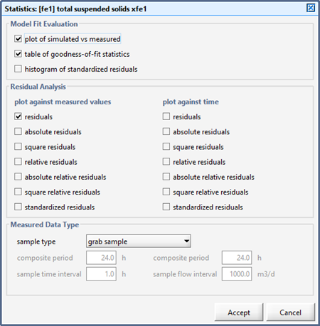
Figure 6‑21 – Selecting the Statistical Analysis to be Preformed on the Model
Note: For full details on the calculation of all the statistical analysis available in GPS-X, refer to the Technical Reference manual.
26. Press Accept. GPS-X will automatically produce the selected plots on the current output tab. Press the Auto Arrange button on the Output toolbar to view all of the plots.
Using the data presented in the output plots, you can judge the ability of your model to represent data collected from your plant. If you are not satisfied with the statistical analysis, further manipulation to influent advisor and your object settings may be required. You can use input controllers to fine tune your model within Simulation Mode.
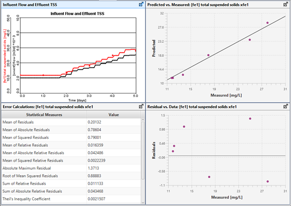
Figure 6‑22 – Results of the Total Suspended Solids Statistical Analysis
The measured data of distributions within a unit can also be plotted along with the simulated result as a bar chart. The methodology for doing so is similar to the previous section.
27. Create a new blank output tab by clicking on the New Graph Tab button on the output toolbar.
28. Create a new graph. For this example, we will use the variable for readily degradable soluble substrate in reactors within the plug-flow tank. Right-click on the plug-flow tank and select Output Variables > Concentrations in Reactors form and within the sub-heading Organic Variables select the More… form. Drag the “readily degradable soluble substrate in reactors” variable under the Soluble Organic Compounds sub-heading to the new tab area. Since it is an array of values, the default graph type is a bar chart.
|
|
29. To open the Data File organizer window, press the Data File button on the main toolbar in GPS-X. |
30. Press the New button to open the Data File Creation Wizard.
31. Select Output Variables in the ‘Input or Output’ pane of the Data File Creation Wizard. Press Next.
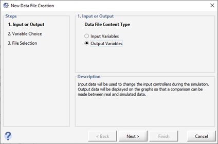
Figure 6‑23 - Select Output Variables in the Data File Creation Wizard
32. Select the Variables. All of the output variables that are currently on an output graph will be available to add to a data file.
Select the following variables:
· [mlss(1)] readily degradable soluble substrate in reactors
· [mlss(2)] readily degradable soluble substrate in reactors
· [mlss(3)] readily degradable soluble substrate in reactors
· [mlss(4)] readily degradable soluble substrate in reactors
Or simply select:
· [mlss] readily degradable soluble substrate in reactors
Note the brackets containing numbers beside the cryptic variable name. This represents the reactor number within the aeration tank. The default number of reactors is four.
Press Next.
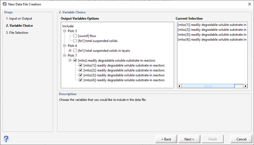
Figure 6‑24 - Select the Output Variables to be Included in the Data File
33. Press Finish to save the File. When prompted to open the new Excel sheet press Yes.
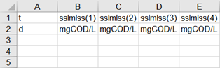
Figure 6‑25 - Output Variable Data File Created by Data File Creation Wizard
34. Use the data in the table below to populate the Data File. Save the Excel Sheet.
Table 6‑3 – Measured Data for Aeration Tank
|
t |
sslmlss(1) |
sslmlss(2) |
sslmlss(3) |
sslmlss(4) |
|
d |
mgCOD/L |
mgCOD/L |
mgCOD/L |
mgCOD/L |
|
0 |
2.8 |
1.68 |
1.21 |
0.88 |
35. Add the data file. Following the same procedure as the previous section where we added an input data file to the layout, access Scenario > Configuration / Data Files and add this new file to the layout.
36. Autoscale the Bar Chart. Press the ‘Output Properties’ button on the Outputs toolbar and select the Autoscale feature for the Bar Chart.
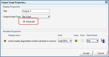
Figure 6‑26 – Autoscale the Bar Chart
37. Run a 0-day simulation with Steady-State clicked ON. The data from the Excel file should show up with the simulated result as a bar chart, as shown in Figure 6‑27.
Notice that the simulated result is shown as a colored bar chart and the measured data is shown as a meshed bar chart.
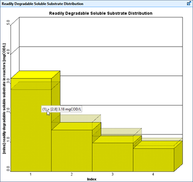
Figure 6‑27 – Bar Chart showing Measured Data
Clicking on a bar will display the measured data (in square brackets) followed by the simulated data value.
38. Save the layout.
Automatic process control is well established in many applications ranging from large refineries using multivariate model-based control to climate control of buildings using simple on/off control. Wastewater treatment plants are no exception. The implementation of even basic automatic control should improve performance and save money. In GPS-X, the user can simulate the effects of automatic process control.
To improve and stabilize operation, as well as realize energy savings, you decide to implement MLSS and dissolved oxygen control. You will do this by incorporating MLSS and DO controllers into your system.
This tutorial will show you how to set up a dissolved oxygen controller that automatically changes the aeration rate to meet the dissolved oxygen set point.
This tutorial also will show you how to set up an MLSS controller to automatically adjust the biosolids wastage rate to meet the specified MLSS set point.
1. Open the layout completed in Tutorial 2 and save it as `tutorial-7’.
2. Check that the DO Controller is activated. By default, the aeration tank is set up to use a DO controller, but we will just confirm that it is selected. Within the Simulation mode for the Aeration Tank go to Input Parameters > Operational and in the Aeration Setup section, the specify oxygen transfer by… variable should be set to Using a DO Controller. If it isn’t, switch to modelling mode, change the value and come back to simulation mode.
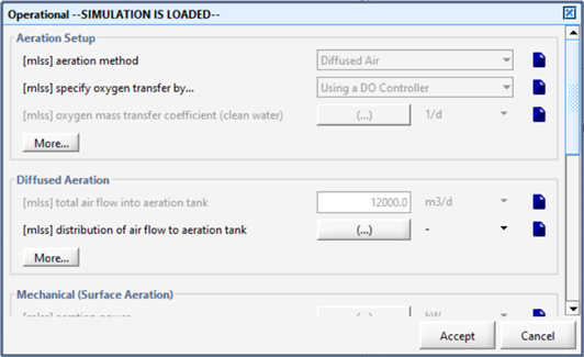
Figure 7‑1 – Check that DO Controller is On
3. Create new input controls. On a new input tab, you will create sliders for two of the DO setpoints. The setpoints can be accessed from the aeration tank’s Input Parameters > Operational form under the Aeration Control section.
Click the ellipsis button (…) beside the DO setpoint label to access the individual array elements.
Drag the first and last DO setpoint array elements to the input control tab to create the sliders.
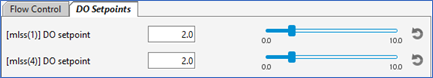
Figure 7‑2 – DO Setpoint Input Controllers
4. Create a new output graph. You will be adding the dissolved oxygen concentration in the first and fourth reactors of the plug-flow tank and the effluent ammonia nitrogen.
Right-click on the aeration tank and select the Output Variables > Concentrations. Beside the dissolved oxygen in reactors label click the ellipsis button (…) to access the individual array elements. Drag the first and last elements to a new graph (both elements are to be contained in the same graph).
Right-click on the aeration tank’s effluent stream (not the tank itself). Select Output Variables > Concentrations and drag ammonia nitrogen (under the Nitrogen Compounds section) to the graph.
5. Edit the graph settings. Change the max value of the y-axis to 10 (the same as the DO setpoint slider limit) and give the graph a proper title.
6. Auto Arrange the graphs.
7. Save the layout.
8. Run some 20 day simulations, varying the influent flowrate and the DO setpoints.
Now we are going to add an MLSS controller to the layout to automatically adjust the biosolids wastage rate to meet the specified MLSS set point.
9. Switch to Modelling Mode.
10. Locate the control variable. This will be the MLSS in the aeration tanks’s effluent stream. We will need to discover the cryptic name (ie. the internal “short form” variable name within GPS-X calculations) of this variable so that we can identify this variable later.
Right-click on the aeration tank’s effluent stream (not the tank itself) and select Output Variables > Concentrations. You should see a form like Figure 7‑3.
Hover the mouse pointer over the label for mixed liquor suspended solids and a tooltip should appear. The tooltip has the form label/cryptic. From this, we can see that the cryptic name of the variable is xmlss. Remember this value for later.
Alternatively, you can right-click on the label for mixed liquor suspended solids and select “Copy Cryptic Name to Clipboard”. This will store xmlss on your computer’s clipboard so that you can paste it into a field later.
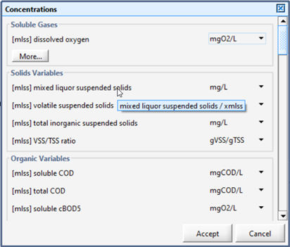
Figure 7‑3 – Viewing Cryptic Variable Name
11. Identify the manipulated variable. The most logical variable for this is the wastage flowrate, which in this case, is the pumped flow from the clarifier.
12. Turn on the controller. Access the clarifier's Input Parameters > Operational data entry form. You will be changing a couple of values in this dialog.
Under the Pumped Flow section, turn on the controller and set the setpoint for control variable to 2000.
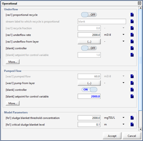
Figure 7‑4 – Clarifier’s Operational Dialog (Pumped Flow)
13. Define the control variable. At the bottom of the Pumped Flow section (see figure above), click the More… button to access the controller’s settings (Figure 7‑5).
· replace blank with xmlss in the control variable field (use Ctrl-V to paste the cryptic name if you had previously saved it to the clipboard)
· enter 0.05 days as the controller sampling time (this represents the frequency with which the controller samples the control variable, or MLSS in this case)
· turn OFF the controller effect on control variable - direct. This means that the manipulated variable, the wastage flow rate, is increased to reduce the control variable, MLSS. (A different control loop such as air flow and DO concentration would require the controller effect on control variable - direct switch to be turned ON as an increase in the manipulated variable, air, would result in an increase in the control variable, DO). (ie. Turn OFF for an inverse relationship and turn ON for a proportional relationship)
· enter 200 m3/d as the maximum pumped flow
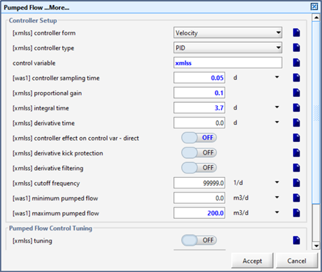
Figure 7‑5 – MLSS Controller Settings
14. Accept the forms.
15. Save the Layout.
16. Switch to Simulation Mode.
17. Create a new input tab. You’ll be adding 5 input controllers to the tab.
These settings can be found by going to the clarifier’s Input Parameters > Operational > Pumped Flow main form and within the Pumped Flow More… form.
· controller on/off
· setpoint for control variable (set limits from 0 to 4000)
· proportional gain (set limits from 0 to 50)
· integral time (set limits from 0 to 10)
· derivative time (set limits from 0 to 10)
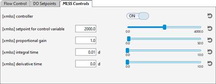
Figure 7‑6 – MLSS Input Controls
18. Create a new graph. Add the following three variables to the same graph:
· the mixed liquor suspended solids (from the aeration tank’s effluent stream Output Variables > Concentrations form)
· the influent flow (from the influent’s Output Variables > Flow form)
· the wastage flow (from the clarifier’s pump stream Output Variables > Flow form)
19. Edit the graph properties. Change the max values of the y-axis to 5000 (influent flow), 5000 (mlss), and 600 (wastage flow).
Note that you may have to ‘unlock’ the max fields so that you can edit the values individually (click the lock icon beside the Max label).
Give the graph an appropriate title.
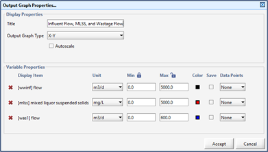
Figure 7‑7 – Graph Properties
20. Create a scenario. Call it “Sinusoidal” and change the influent flow type to sinusoidal and keeping the influent flow as the default 2000.0 m3/d (Tutorial 3 - Using Scenarios for instructions if needed).
21. Save the layout.
22. Run a 10-day dynamic simulation with sinusoidal scenario and the controller turned ON.
Initially, you will find that the manipulated variable, the wastage flow rate, oscillates wildly between its minimum and maximum values. This is a controller tuning problem. It is usually possible to obtain reasonable controller performance by trial and error. In this example, one may conclude that the controller gain is too large. One option for tuning this controller by trial-and-error is as follows:
· Start with a low proportional gain (0.001), high integral time (10 days), and low derivative time (0 days). This creates a sluggish but stable controller.
· Watch how the wastage rate changes to counteract the effect of a disturbance (e.g. influent flow rate). If it does not react quickly enough, try increasing the proportional gain. Continue to increase the proportional gain until you get a reasonably responsive control effect, but still a stable response.
· If the wastage rate becomes unstable (wild oscillations) decrease the proportion gain.
· With the proportional effect stable, try decreasing the integral time to increase the performance of your controller.
· If there is too much overshoot, try increasing the derivative time
A simplified understanding of the three elements of a PID controller is: fast, persistent and predictive for the P, I and D terms respectively. Remember that automatic process control is not a simple subject and it may not be possible to achieve the level of control that you desire. Consider the process time constant of the MLSS in the aeration basin. It takes several days for a plant to reach a new steady-state given a change in wastage rate, while the plant upsets (changes in the influent flow rate) that can have a dramatic effect on the MLSS can occur in a matter of hours or even minutes.
There are several published approaches for finding good initial tuning constants for PID controllers. One approach is to use the Ciancone correlations (Marlin, 1995[i]) which are included in GPS-X's PID tuning tool. The Ciancone correlations provide the tuning constants given the gain, time constant, and dead time of the process, under the assumption that the process dynamics may be represented with reasonable accuracy by a first-order plus dead time model. In GPS-X's PID tuning tool, the process response to a step change in the manipulated variable is fit to a first-order plus dead time model using least squares (in tuning mode). The Ciancone correlations are then used to determine the appropriate values for the tuning constants.
23. Create another scenario. Base it on the Sinusoidal scenario (so that it has the influent flow type from that scenario) and call it “Tuning”.
24. Activate the pumped flow control tuning mode.
Browse to the clarifier’s Input Parameters > Operational form. Click the Pumped Flow section’s More button and find the Pumped Flow Control Tuning section.
Turn the tuning switch ON. Also drag this variable to the input control tab so that it can be easily turned OFF in the future.
The fractional step size can be specified on that form and can be a positive or negative value. In this case, set the fractional step size to 0.5.
Accept the More dialog to return to the Operational form.
Now (under the Pumped Flow section) turn the controller OFF and set the pumped flow value to 100 m3/d.
This fractional step size corresponds to a step in pumped flow rate from 100 m 3 /d to 150 m 3/d.
Accept the Operational form.
25. Double-check that you have the right settings. Select Scenario > Show from the Simulation Toolbar to see all of the variables that you have changed for this scenario. You should see a dialog similar to Figure 7‑8.
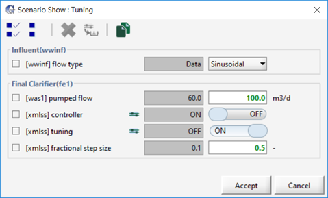
Figure 7‑8 – Scenario Show Dialog
26. From the input controls tab, turn the MLSS controller ON and run a 0-day steady state simulation with the newly created scenario.
27. Now, turn the MLSS controller OFF using the ON-OFF control switch[4] and run a 10-day dynamic simulation.
![]()
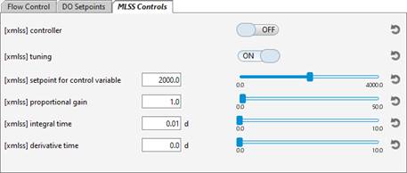
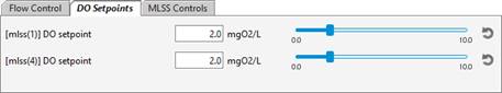
![]()
Figure 7‑9 - Input Controller Setting
The simulation performed in tuning mode is shown in Figure 7‑10. The essential characteristics of a successful tuning mode simulation are:
· It must be started under steady-state, with values of the manipulated (pumped flow) and controlled (MLSS) variables representative of normal operating conditions.
· The simulation should last long enough to capture most of the process dynamics (i.e. the simulation should end at steady-state, or be approaching steady-state), and
· The step in the manipulated variable should be large enough to dominate other "noise" that affects the controlled variable (in this case the sinusoidal influent flow pattern).
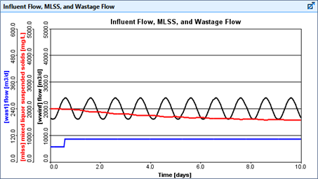
Figure 7‑10 – Tuning Mode Simulation
At the end of the simulation, PID tuning constants will be calculated (this may take several seconds), and will appear in the Command Window (see Figure 7‑11).
|
|
The Command Window can be opened by selecting this option from the Simulation Control button on the Simulation Toolbar. Scroll to the bottom of the Command Window for the xmlss settings displayed in Figure 7‑11. |
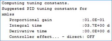
Figure 7‑11 – Calculated PID Tuning Constants
28. Create another scenario. Base it on the Tuning scenario (so that it starts with all the variables from that scenario) and call it “MLSS Control”.
29. Change the input controller values. In the input control tab, set the proportional gain, integral time, and derivative time to the values shown in the Command Window. Also turn ON the MLSS controller and turn OFF the tuning mode.
|
|
30. Transfer the controller values to the scenario. Press the “Transfer controls to scenario” button on the Controls toolbar and add the controller tuning constants to the scenario to store these settings. |
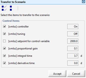
Figure 7‑12 – Transfer to Scenario
31. Save the layout.
32. Run a 10-day simulation. The results shown in Figure 7‑13 were performed using these tuning parameters for the MLSS controller. The MLSS setpoint was 2000 mg/l and the average influent flow rate was decreased to test the performance of the controller under dynamic conditions.
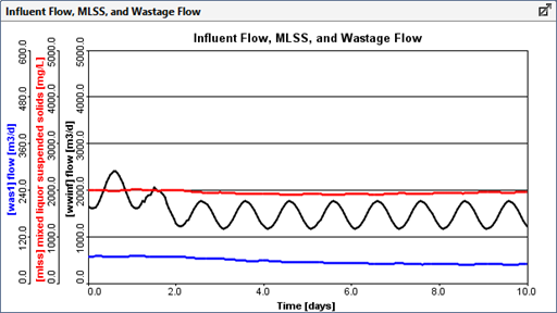
Figure 7‑13 – Simulation with MLSS Controller
Some important operational variables in a wastewater treatment plant are site specific and difficult to generalize. These variables include sludge residence time (SRT) and food-to-microorganism ratio (F/M). In addition, other calculations, such as daily averages, moving averages, and mass flows are applied to most water quality parameters throughout the plant. Consequently, it is desirable for any wastewater treatment plant model to contain these traditional process variables, and GPS-X provides you with this capability
This tutorial will show you how to define operational variables such as SRT.
In addition, mathematical operations such as averaging and flux calculations will be demonstrated.
These operations are centered around the Define function (Tools > Define menu or the Define button located on the main toolbar).
1. Create a new layout consisting of:
· A wastewater influent object,
· a control splitter,
· a plug-flow tank,
· a rectangular secondary clarifier
· a 2-flow combiner
· a wastewater outfall
Use the mantis2lib library and the default model selections (codstatesinfluent model, the mantis2 plug flow tank model and the simple1d rectangular clarifier model).
Connect the unit processes and add the labels as displayed in Figure 8‑1. The control-splitter unit process will be used to simulate a bypass weir.
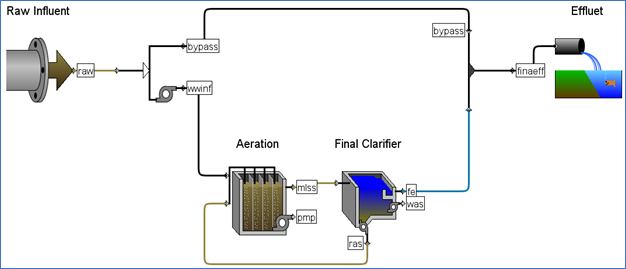
Figure 8‑1 – Tutorial 8 Layout
2. Modify the clarifier underflow parameters. Access the Input Parameters > Operational data entry form and change the following settings:
· Turn ON the proportional recycle.
· Beside stream label to which recycle is proportional change “blank” to “wwinf” (ie. the influent stream to the aeration tank).
· The recycle fraction is already 0.8 which is acceptable for this example.
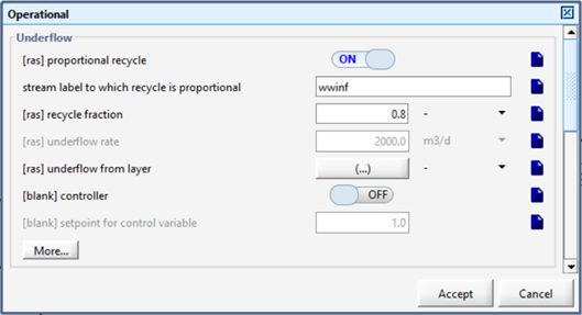
Figure 8‑2 – Modify Underflow Settings
3. Modify the clarifier pumped flow. In the same data entry form (scroll down if necessary) change the pumped flow (which will be used as the wastage rate) from 40 m3/d to 100 m3/d.
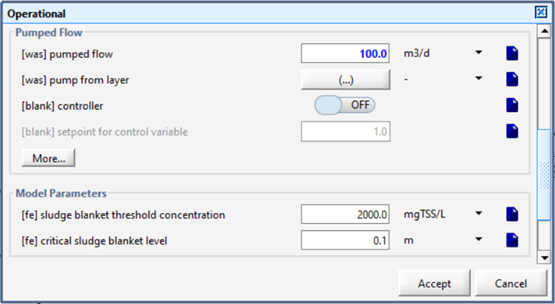
Figure 8‑3 – Modify Pumped Flow
4. Accept these changes and save the layout.
Now that the layout has been set up, we will define a mass flow variable of the effluent solids. This mass flow is defined as the effluent suspended solids multiplied by the effluent flow rate.
5. Access the Define Wizard. Click on Define button on the main toolbar and select Mass Flow from the options.
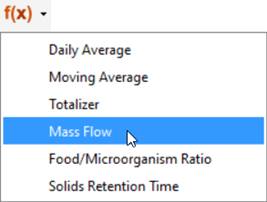
Figure 8‑4 – Mass Flow in the Define Wizard Submenu
6. Select the streams (as shown in Figure 8‑5):
· Control Splitter > bypass
· Final Clarifier > fe
· 2-flow Combiner > finaleff
7. Select the variable. As shown in Figure 8‑5, select Composite Variables > total suspended solids.
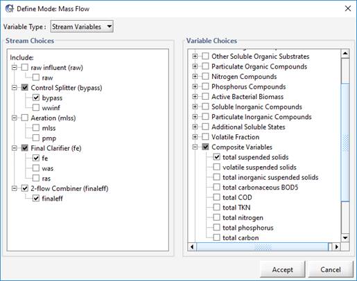
Figure 8‑5 – Define Mass Flow Wizard
8. Press Accept and then save the layout.
Now that the variable has been defined, we will set up a graph and run a simulation to view the results.
9. Switch to Simulation Mode.
10. Create a new graph. You will be adding three mass flow variables to this graph.
Right-click on the clarifier fe connection point and select the Output Variables > Defined Variables > Mass Flow.
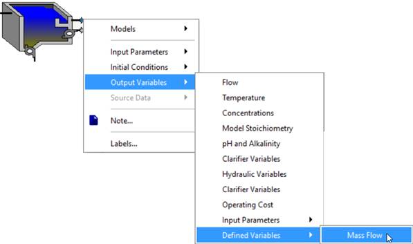
Figure 8‑6 - Accessing the Defined Variables
Drag the Mass Flow.total suspended solids variable to an output graph.
Repeat this procedure for the bypass and the finaleff streams so that all three mass flows are displayed on the same output graph.
11. Modify the graph settings. Set the max axis values on that graph to 1,000 kg/d and set the title to “Mass Flows”.
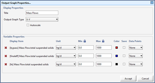
Figure 8‑7 - Mass Flow Graph Settings
12. Create an input controller for the influent flow rate. As described in Tutorial 2set up the controller and set the maximum flow to 10,000 m3/d.
13. Auto Arrange the graph and run a 20-day dynamic simulation.
14. Increase the influent flow rate and notice that when the influent flow rate is above 2000 m3/d (the default pump flow rate for the Control Splitter object), some flow will begin to bypass the plant and show up in the bypass stream. An example is displayed in Figure 8‑8. Note that your output graph will look different when compared to the figure below depending on the adjustments you make to the slider during the simulation run.
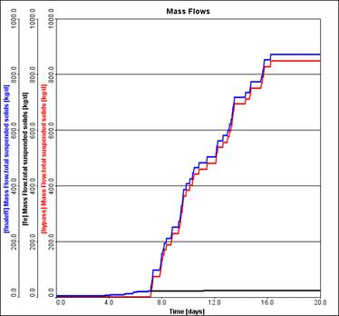
Figure 8‑8 – Mass Flow Output Graph
15. Try changing the bypass flow limit by increasing the pumped flow rate in the Control Splitter object. To prevent having to recompile the model, this must be done either by defining a scenario or by placing the bypass pump flow on an input controller. For instance, to create an input controller, right-click on the control splitter and go to Input Parameters > Pumped Flow and add pumped flow as an input controller.
16. Re-run the simulation and try to reduce the total mass flow of solids discharged to the receiving water.
17. Save the layout.
In this section, you will learn how to calculate and display SRT, the solids residence time in the system.
18. Switch to Modelling Mode.
|
|
19. Access the SRT Manager window. Click on Define button on the main toolbar and select Solids Retention Time from the options. |
|
|
20. Create a new SRT Variable. Click the green ‘+’ button and enter ‘tank’ as the name for the variable (Note: the full name will be ‘srttank’ because ‘srt’ is automatically prepended to all variable names). |
21. Access the SRT Manager window. Click on Define button on the main toolbar and select Solids Retention Time from the options.
22. Create a new SRT Variable. Click the green ‘+’ button and enter ‘tank’ as the name for the variable (Note: the full name will be ‘srttank’ because ‘srt’ is automatically prepended to all variable names).
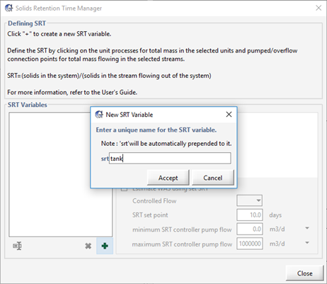
Figure 8‑9 – Create a New SRT Variable
23. Accept the name. A new blank SRT equation will be shown on the right side of the window.
24. Define the equation. This process involves clicking on the appropriate locations on the drawing board while keeping the SRT Manager window open. You may have to move the SRT Manager window in order to access everywhere that you need.
There are two parts to the SRT equation: Mass()/Mass Flow()
I. The numerator is the mass section of the equation, and it includes the mass of solids held in each tank. Typically, SRT calculations only include the mass of solids held in the aeration basin, but it is also possible to calculate SRT by summing the mass in the aeration basin and the final clarifier. While the SRT equation is shown, every time you click on a tank the mass of solids in that unit process will be included in the SRT calculation.
Click the following processes to add them to the numerator:
|
|
· Aeration Tank (since this process represents several reactors, you will be prompted for which ones you’d like to include. Include all of them.) · Clarifier |
II. The denominator part of the equation is the excess solids mass flow lines that are used to calculate SRT. This is done by pointing to the flow lines which convey solids out of the system. Typically, this will only include the waste flow.
Click the following connection points to add them to the denominator:
|
|
· was · fe |
The equation should now look like the following:
Mass(mlss,fe)/Mass Flow(was,fe)
However, for this example, we will not be including the clarifier’s mass in the calculation.
25. Remove the clarifier’s mass. Click on the clarifier again to remove it from the equation.
Mass(mlss)/Mass Flow(was,fe)
26. Close the SRT Manager window to accept the equation.
27. Save the layout.
28. Switch to Simulation Mode.
29. Create a graph with the SRT variable. In Simulation Mode, when you open the SRT Manager from the Define menu, you can only view the SRT variables and their equations. You can also drag the variable’s label from this window to a new or existing graph. Drag the ‘srttank’ variable to a new graph.
Note: This will add two variables to the graph. The instantaneous and dynamic SRT. Depending on the need, one or the other can be removed. In our case, we’ll just leave both.
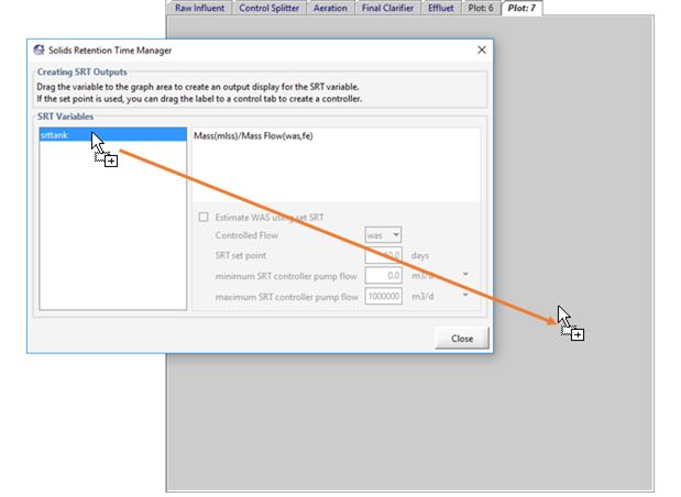
Figure 8‑10 – Dragging SRT Variable to a Graph
30. Modify the graph properties. Change the y-axis max value to 30 days and change the graph title to “SRT”.
31. Save the layout.
32. Try running a few simulations, observing the SRT as you change the amount of solids being wasted out of the system. Do this by adding an input controller for the [was] pumped flow from the secondary clarifier through right-clicking on the was output and going to Input Parameters > Operational.
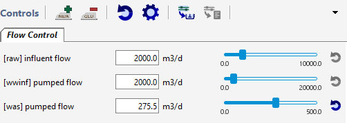
Figure 8‑11 – Update Set of Input Controllers
The procedure for defining averages is similar to setting up mass flow calculations. In addition, averaging calculations can also be applied to a defined mass flow, SRT, or F/M ratio. Here, you will apply averaging calculations to the Mass Flow in the discharge stream defined above.
33. Switch to Modelling Mode.
|
|
34. Access the Define Wizard. Click on Define button on the main toolbar and select Daily Average from the options. |
35. Change the Variable type to “Define Variables.”
Select the desired variable(s). In this case, we will only select 2-flow Combiner > finaleff > Mass Flow > Mass Flow.total suspended solidsas shown in Figure 8‑12.
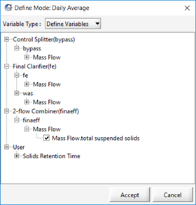
Figure 8‑12 – Define Daily Average Wizard
36. Press Accept and then save the layout.
You have now set up a daily average calculation for the mass flow of suspended solids in the “finaleff” stream.
37. Define a moving average for the Mass Flow.total suspended solids in the “finaleff” stream. Use the same procedure as above except select Moving Average instead of Daily Average from the Define menu.
38. Press Accept and then save the layout.
39. Switch to Simulation Mode.
40. Create a new graph. You will be adding the new daily and moving averages variables to this graph.
Right-click on the combiner’s finaleff connection point and select the Output Variables > Defined Variables > Daily Average and drag the variable to a blank area to create the graph. Do the same with the Moving Average variable and add it to the same graph.
|
NOTE: You will notice in the display form for the Moving Average variable that a number will appear to the right of the variable name. This number represents the number of days that are used in each moving average calculation. You must be in Modelling mode to edit this # of Days value.
Figure 8‑13 – Moving Average # of Days |
41. Change the graph properties. Set a maximum limit of 1,000 kg/d for both variables.
42. Run the model and change the influent flow rate to observe the moving and daily averages. For example, running the model with the following controller settings provides the graph displayed in Figure 8‑14. Note that your output graph will look different depending on how the control slider for the influent flow is adjusted during the simulation.
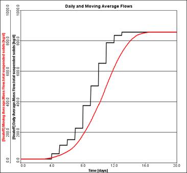
Figure 8‑14 – Moving and Daily Averages Output Graph
When defining a SRT equation, you have the option to create a process controller for SRT. This controller will adjust the waste flow rate to achieve a given SRT set point.
43. Switch to Modelling Mode.
44. Set the SRT controller. Bring up the SRT Manager window. Select an SRT to control (for this example select srttank), and click on the Estimate WAS using set SRT option, as shown below.
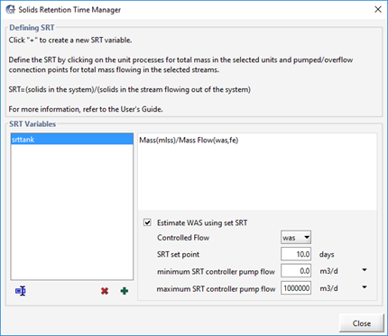
Figure 8‑15 – Estimating WAS using set SRT
45. Edit the settings. In this situation, we are just going to leave the values at their defaults, but in the settings section, you can choose the appropriate wastage flow to control and enter the desired SRT (in days) into the SRT set point field, as well as specify the min/max of the flow.
Only one SRT can be controlled at a time via this method. If multiple SRT controllers are required (e.g. for plants in parallel) then a PID control loop can be used in the pump control section of the secondary clarifier or a toolbox object. More information regarding PID controllers is presented in Tutorial 7.
46. Switch to Simulation Mode.
47. Create another input controller. Open the SRT Manager again (in Simulation Mode) and drag the SRT set point to the input controller tab to create a slider for that variable. Edit the settings and change the max value to 30 days.
At the same time, within the SRT Manager window drag the Estimate WAS using set SRT selection to the input controller tab to create an ON/OFF switch. If desired, this allows you to easily adjust this setting without having to open the SRT Manager in the Modelling mode. For the next steps, keep the use set point SRT to estimate waste flow to ON.
48. Create an output graph. To observe the required WAS flow rate while changing the SRT set point, we will create another graph (on the same tab as the SRT graph) that contains the WAS flow rate. It is accessed by clicking on the clarifier’s WAS connection point and selecting Output Variables > Flow. Edit the graph settings, give the graph an appropriate name and change the max value of the y-axis to 500 m3/d.
49. Try running simulations at various SRT point values to observe required WAS flowrate to achieve the desired SRT. An example is shown below in Figure 8‑16. Note that your output will look different depending on how the SRT set point controller is adjusted during the simulation.
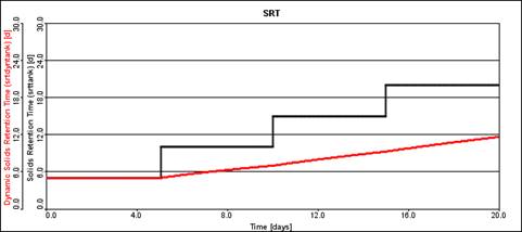
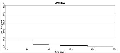
Figure 8‑16 – SRT and WAS Flow Output Graph
With any model, one of the first exercises to carry out is a sensitivity analysis of the model parameters. There are two reasons for doing so: 1) to validate the model results and 2) to identify parameters to be adjusted during calibration. The former reason should allow the modeler to develop some confidence in the model so that it behaves in an expected manner. For example, lowering the air flow rate to the aeration basin should result in a lower dissolved oxygen concentration. The latter reason for performing a sensitivity analysis, parameter identification, is useful because it helps determine the parameters that have the most impact on the model response. We do not want to adjust parameters during a calibration run that have little effect on the model behavior.
After the model is calibrated and verified, sensitivity analyses are useful for other reasons. Mathematical models can be revealing, sometimes allowing us to explore operational strategies that might never have been contemplated otherwise.
In this chapter, you will explore the steady-state and dynamic sensitivity of a basic model.
The purpose of this tutorial is to see how we can extract as much information as possible from a GPS-X model. By the end of this tutorial you should have developed a working knowledge of the Analyze functions. This includes setting up and running steady state, phase dynamic, and time dynamic sensitivity analyses. By completing this tutorial, you will also learn how to interpret the results from these simulations.
The Analyze module is an optional feature of GPS-X. If you have not purchased this module, contact us for pricing information.
Because this feature requires multiple simulations, for demonstration purposes the work will be carried out on a simple model consisting of an influent, a completely-mixed tank, and a rectangular final clarifier.
1. Create a new layout.
2. Select the Comprehensive (mantis2lib) from the Library menu (if it isn’t already selected) (see Figure 9‑1)

Figure 9‑1 – Select Library
3. Create the layout as shown in Figure 9‑2 with a codstates Wastewaterinfluent model, mantis2 Completely-Mixed Tank(CSTR) model and simple1d Rectangular Secondary Clarifier model. These should be the default model settings.
4. Save the layout with the name ‘tutorial-9’.
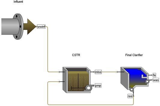
Figure 9‑2 – Tutorial 9 Layout
5. Switch to Simulation Mode.
6. Create a new scenario. Call it ‘Sinusoidal’.
7. Change influent parameters. Access the influent’s process menu and change:
· Flow > Flow Data > flow type parameter to Sinusoidal.
· Flow > Flow Data > influent flow parameter to 5,000 m3/d.
· Composition > Load Type Options > loadtype parameter to Sinusoidal.
8. Change CSTR parameters.
· Set Input Parameters > Operational > specify oxygen transfer by to Entering Airflow.
· Set the air flow into aeration tank to 15,000 m3/d.
9. Create input controls. Place the influent flow and the air flow into aeration tank on an input control tab. They can be found in the following locations:
· the influent flow variable can be found in the influent object Flow >Flow Data
· the air flow into aeration tank can be found in the CSTR object Input Parameters > Operational
Put both parameters on the same input control tab, with limits of 2,000-10,000 m3/d for the influent flow and 10,000-40,000 m3/d for the air flow.
10. Create output graphs. You will create four different graphs. One for each of:
· ammonia nitrogen (from the clarifier’s effluent stream’s (fe) Output Variables > Concentrations form)
· total carbonaceous BOD5 (from the clarifier’s effluent stream’s Output Variables > Concentrations form)
· total nitrogen with soluble dintrogen gas (from the clarifier’s effluent stream’s Output Variables > Concentrations under the Nitrogen Variables heading select the More… form)
· dissolved oxygen (from the CSTR’s Output Variables > Concentrations form)
Use limits of 0-30 mgN/L for NH3-N, 0-200 mgO2/L for cBOD5, 0-100 mgN/L for total nitrogen and 0-5 mgO2/L for DO.
11. Auto arrange the graphs.
12. Save the layout.
You will now carry out a steady state sensitivity analysis of the air flow into the aeration tank on the dependent variables that you have selected for display (NH3-N, cBOD5, total nitrogen, DO).
13. Set up the independent variable. Open the settings window for the input controls and change:
· the Type of controller for the air flow into aeration tank to “Analyze-Step”.
· the Delta value to 500. This is the increment that the analyzer will step through from the min to max values.
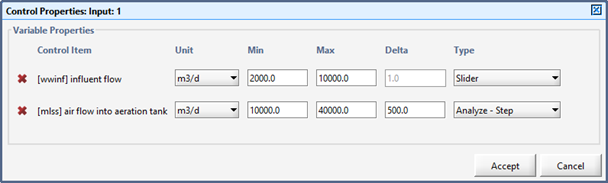
Figure 9‑3 – Setting up the Independent Variable
|
|
14. Confirm the analysis type. Click the little arrow beside the Analyze button on the main toolbar (or access it through the main menu’s Tools > Analyze) and confirm that “Steady State” is selected. |
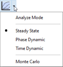
Figure 9‑4 - Selecting Analysis Type
15. Switch to Analyze Mode. Click the Analyze button on the main toolbar (or access the Analyze Mode checkbox through the main menu’s Tools > Analyze) to turn on the analyzer.
The status bar at the bottom of the main window will indicate that you are in Analyze Mode and the graphs will change so that the independent variable is the x-axis instead of time.
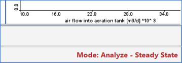
Figure 9‑5 – Status Bar showing “Analyze – Steady State” Mode
16. Run a steady state 0-day simulation.
Observe the effect of an increase in the air flow on DO and the effluent BOD5, NH3 and total nitrogen. Typical results are shown in Figure 9‑6.
Note that an air flow of 40,000 m3/d results in a DO level over 2.0 gO2/m3.
Try the analysis using different influent flows.
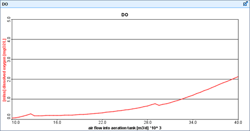
Figure 9‑6 – Steady State Analysis Results
You will now carry out a time dynamic sensitivity analysis of the air flow into the aeration tank on the dependent variables that you have selected for display (NH3-N, cBOD5, total nitrogen, DO).
|
|
17. Change the analysis type. Click the little arrow beside the Analyze button on the main toolbar (or access it through the main menu’s Tools > Analyze) and change the type to “Time Dynamic”. |
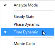
Figure 9‑7 – Selecting Analysis Type
18. Switch to Analyze Mode. If you aren’t already in analyze mode (check on the status bar), click the Analyze button on the main toolbar (or access the Analyze Mode checkbox through the main menu’s Tools > Analyze) to turn on the analyzer.
The status bar at the bottom of the main window will indicate that you are in Analyze – Time Dynamic mode. The graphs will have time as the x-axis, just like in the regular simulation mode.
Figure 9‑8 – Status Bar showing “Analyze – Time Dynamic” Mode
19. Set the simulation time to 1-day (with Steady State checked so that the initial conditions are at steady state) and Start the simulation. The results of this simulation are shown in Figure 9‑9.
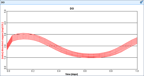
Figure 9‑9 – Example of Time Dynamic Analysis Results
Each successive curve on the various graphs is the result of a dynamic simulation using a specific air flow into the aeration tank. Notice in Figure 9‑9 that for increasing values of air flow, the DO concentration in the aeration tank increases - it also fluctuates over time because of the sinusoidal influent flow and load patterns. You can change the number of run curves on the graph by going to View > Preferences > Input/Output > Number of runs displayed (analyze/optimize).
You will now carry out a phase dynamic sensitivity analysis of the air flow into the aeration tank on the dependent variables that you have selected for display (NH3-N, cBOD5, total nitrogen, DO).
20. Select Phase Dynamic from the Analyze drop-down menu.
21. Set the Simulation time to 1-day (with Steady State checked so that the initial conditions are at steady state) and Start the simulation.
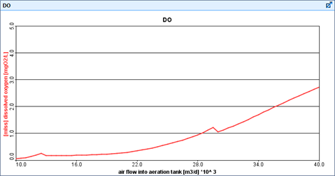
Figure 9‑10 – Example of Phase Dynamic Analysis
This type of analysis allows you to run the same dynamic simulation as in the previous step. The only difference is in the graphical display. Here the results will be plotted against the analyze variable and not against time. The length of the simulations will set the phase. Typical results are shown in Figure 9‑10 for a sinusoidal influent.
In this case, the results are very similar to the Steady Stateanalysis type since the simulation was not very dynamic.
The graph shows the DO concentration after 1.0 day for an air flow of 10,000 to 40,000 m3/d (as opposed to showing the steady-state value at time t=0 when carrying out the Steady State analysis.)
Model calibration and verification is one of the most important components of any modeling project. Model calibration, also known as parameter estimation, is defined as the process of adjusting model parameters such that the difference between observed and simulated results is minimized. For example, if the difference between observed and simulated effluent suspended solids is too large, it is likely that you will want to adjust some of the model parameters.
GPS-X provides a very convenient way of adjusting the model parameters, based on a non-linear dynamic multi-parameter optimization algorithm (Nelder-Mead simplex method).
In this example, the estimation of two kinetic parameters (heterotrophic growth rate and half saturation constant) is carried out in order to fit the model-predicted soluble substrate concentration with the measured data. Although this is a simple example, using only a CSTR unit process, the procedure outlined below is the important subject.
The purpose of this tutorial is to develop a basic understanding of parameter estimation using GPS-X. After this tutorial, you will be able to target variables that you are interested in fitting to the data, select the model variables to be adjusted and specify the form of the objective function. Other optimizer variables such as termination criteria and number of data points will be explained in this tutorial.
1. Start a new layout.
2. Switch to the Carbon, Nitrogen (cnlib) library.
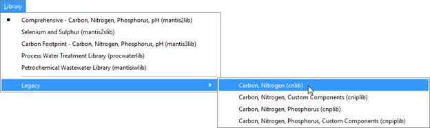
Figure 10‑1 – Switch Library to cnlib
3. Drop a single Completely-Mixed Tank on the drawing board. Confirm that the process model is mantis. The stream labels will be left at their defaults (should be the numbers 1 to 4).
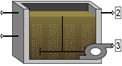
Figure 10‑2 – Simple Layout for Optimization
4. Set the tank’s initial conditions. For this example, we will just access Initial Conditions > Initial Concentrations and change initial readily degradable substrate to 200 mgCOD/L.
5. Change the tank’s parameters.
· Set Input Parameters > Operational > specify oxygen transfer by to Entering Airflow.
· Set the air flow into aeration tank to 40,000 m3/d.
|
|
6. Change the simulation setup parameters. Open the Site Properties window by clicking on the button in the upper left corner of the drawing board. Open the Simulation Setup tab. |
Change the stopping time to 0.25 days, and the communication interval to 0.01 days.
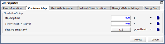
Figure 10‑3 – Changing Simulation Setup
7. Save the layout with the name ‘tutorial-10’.
8. Switch to Simulation Mode.
9. Create a graph. Add readily degradable soluble substrate (from Output Variables > Concentrations > Organic Variables > More…) on a graph and change the limits to 0-300 mgCOD/L.
10. Run a 0.25-day simulation (make sure Steady State is NOT checked). Your output should match that of the graph in Figure 10‑4.
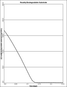
Figure 10‑4 – Readily Biodegradable Substrate Output Graph
You will now optimize two kinetic parameters in order to obtain the best fit between effluent soluble substrate data and simulation results.
11. Create input controls. Place the following parameters (found in the tank’s Input Parameters > Kinetic) on an input control tab:
· heterotrophic maximum specific growth rate
· readily biodegradable substrate half saturation coefficient
Set limits of 0.5-5 d-1 for the growth rate, and 0.5-10 mg COD/L for the half saturation coefficient.
12. Add observed data file. Create a spreadsheet file with the example data listed in Table 10‑1. Save it in the same directory as your layout file, then add it to that layout. If you need a reminder of the process, see Tutorial 6.
Table 10‑1 – Example Data for Optimization
|
t |
ss2 |
|
d |
mgCOD/L |
|
0.00 |
213.5401 |
|
0.01 |
209.4151 |
|
0.02 |
197.8075 |
|
0.03 |
187.389 |
|
0.04 |
172.1104 |
|
0.05 |
185.44 |
|
0.06 |
178.8617 |
|
0.07 |
148.0012 |
|
0.08 |
152.297 |
|
0.09 |
142.1657 |
|
0.10 |
120.4514 |
|
0.11 |
117.4068 |
|
0.12 |
120.551 |
|
0.13 |
95.89756 |
|
0.14 |
84.38476 |
|
0.15 |
79.90364 |
|
0.16 |
73.47583 |
|
0.17 |
47.58231 |
|
0.18 |
39.27833 |
|
0.19 |
28.0756 |
|
0.20 |
16.67731 |
|
0.21 |
4.3656 |
|
0.22 |
0.624523 |
|
0.23 |
1.157525 |
|
0.24 |
0.985331 |
|
0.25 |
1.235542 |
13. Save the layout.
14. Re-run the simulation. Manually change the growth rate and half saturation parameters with the goal of minimizing the difference between the simulated and measured data. Figure 10‑5 displays the initial graphical output prior to making manual changes to the growth rate and half saturation parameters.
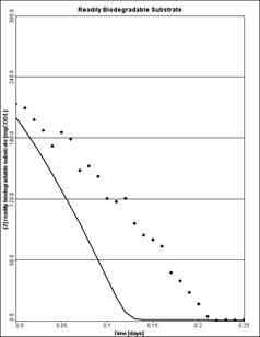
Figure 10‑5 – Readily Biodegradable Substrate Output Graph with Example Data
After manually calibrating the model in the previous section (i.e. adjusting the heterotrophic maximum specific growth rate and readily biodegradable substrate half saturation coefficientparameters using the sliders and re-running the simulation), you will now set up the automatic parameter optimization tool to perform a search routine to find the best set of parameter values to fit the prediction to the measured data.
|
NOTE: It is always advisable to carry out a manual calibration first to determine the effects of parameters on the simulated response before carrying out an optimization. |
15. Switch to Modelling Mode.
|
|
16. Click on the Optimize button on the top toolbar and select Optimize Setup. This will display the Optimizer Setup Wizard. |
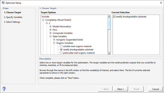
Figure 10‑6 – Optimize Setup Wizard (Target Variables)
17. Select the Target Variable. In this case, it is the readily biodegradable substrate in the reactor. It can be found under:
Completely-Mixed Tank(2) > 2 > State Variables > Organic Variables
18. Click Next to proceed to the next stage.
19. Select the Optimize Variables. These are the input parameters being adjusted during the fitting exercise. Select the following variables:
· heterotrophic maximum specific growth rate
· readily biodegradable substrate half saturation coefficient
These can be found under:
Completely-Mixed Tank(2) > Kinetic > Active Heterotrophic Biomass
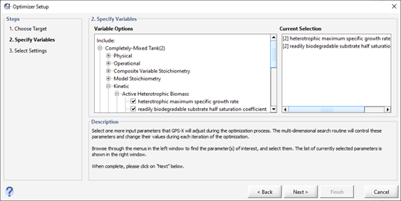
Figure 10‑7 – Optimize Setup Wizard (Optimize Variables)
20. Click Next to proceed to the next stage.
21. Specify Optimizer Settings. The last step in the process is to specify which kind of optimization we are doing. We will use Fit to Data, Time Series, and Maximum Likelihood.
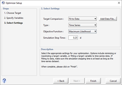
Figure 10‑8 – Optimize Setup Wizard (Optimizer Settings)
We can also use the “Add Data File…” button here to add data if needed, but we have already specified our data file earlier (step 12) so we don’t need to do it again here.
22. Click Finish to complete the set up. Switch to Simulation mode.
Note that a new Input panel has been created with our two Optimize parameters already set to optimize mode. The target variable is also now plotted on a new graph. (These two actions may leave you with tabs with nothing in them. Feel free to delete them).
|
|
23. Enter Optimization Mode. Press the Optimize button on the main toolbar and select Optimize Mode. When optimize mode is active, the optimize icon on the main toolbar will change to display a green checkmark. |
24. Save the layout.
25. Start the simulation. GPS-X will automatically perform a number of simulations in a row, adjusting the values of the two optimize parameters each time to get a better fit to the observed data. Once the simulator has determined that no better fit can be achieved, it will stop. This should only take a few seconds.
At each optimization iteration, GPS-X plots the simulation results (i.e. predicted values) that correspond to the current parameter values. It retains the 7 most recent simulations on the graph. You can change the number of run curves on the graph by going to View > Preferences > Input/Output > Number of runs displayed (analyze/optimize). The simulation results are shown by a black line and the data are shown by red markers.
Note that the initial parameter values used in the optimization are the default values found in GPS-X. The Solution Report, accessed in the Command Window, includes the final parameter values and the results of the statistical tests.
A plot of the fitted model and the measured data is shown below.
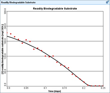
Figure 10‑9 – Results of
Optimization
No wastewater treatment plant modeling/simulation tool can be general enough to automatically handle ALL conceivable plant layouts or desired variables. So, GPS-X facilitates model layout customization. This is an advanced feature of GPS- X and requires a basic understanding of ACSL, the simulation language upon which GPS-X is based. The potential of the tool will be demonstrated using the following simple example.
In this tutorial, you will add two equations to calculate the specific oxygen uptake rate (SOUR) for the first stage of a plug-flow tank. One of the equations will assume an ideal oxygen uptake rate (OUR) measurement and the second will simulate measurement noise on the oxygen uptake rate measurement. This variable is often used for toxicity detection and in process control strategies.
This tutorial is designed to introduce you to the steps
required to input your own code for a specific plant layout.
You will learn how to set up the GPS-X interface, allowing you to
input and output these customized variables as if they were part of
the original layout.
1. Open the layout completed in Tutorial 1 and save it as `tutorial-11’
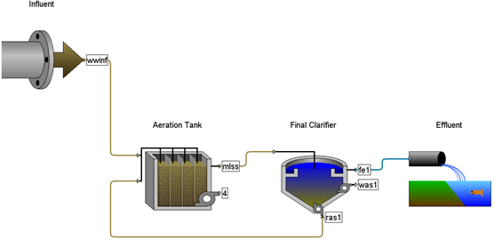
Figure 11‑1 – Tutorial 11 Layout
2. Switch to Modelling Mode.
3. Change the influent’s parameters.
· Set Flow > Flow Data > flow type to Sinusoidal.
4. Change the tank’s parameters.
· Set Input Parameters > Operational > specify oxygen transfer by… to Entering Airflow.
· Set the total air flow into aeration tank to 30,000 m3/d.
5. Save the layout.
7. Create a new graph. You will add the flow and a variable from the first reactor of the plug flow tank to the same graph.
· add flow from the influent’s Output Variables > Flow form
· add actual oxygen uptake rate from the first reactor. This is accessed through Output Variables > Internal Variables. Click the ellipsis button beside the variable to access the individual elements and drag the first element to the graph.
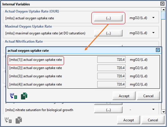
Figure 11‑2 – Accessing Individual Reactor Variables
8. Set the graph properties. In the Output Graph Properties window, set:
· the flow limits to 0-10,000 m3/d
· the OUR limits to 250-1,500 mgO2/L/d
Note: You may have to ‘unlock’ the min/max fields to edit them separately.
9. Save the layout.
10. Run a 10-day dynamic simulation (with the steady-state box checked) to ensure that the model is correctly set up. You should be able to produce a graph similar to Figure 11‑3.
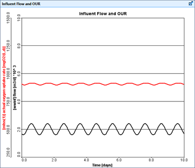
Figure 11‑3 – Example Graph from Dynamic Simulation
11. Switch to Modelling Mode.
12. Open the macros user file. This is done by choosing Layout > General Data > User Files > Macros from the main menu.
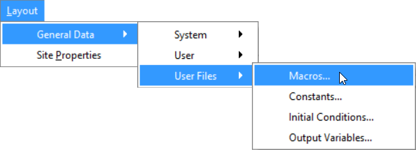
Figure 11‑4 - Accessing the Macro User File
In this file, which is generated when you save the layout for the first time, there are several sections separated by asterisks. They correspond to the different sections of the ACSL program structure. In this example, you will add new code to the DERIVATIVE SECTION as shown below.
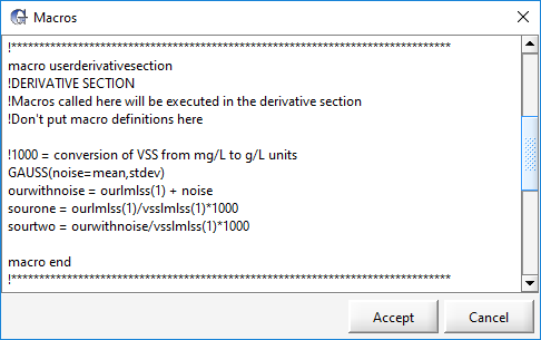
Figure 11‑5 – Adding Code to Derivative Section
13. Add the following code to the DERIVATIVE SECTION:
!1000 = conversion of VSS from mg/L to g/L units
GAUSS(noise=mean,stdev)
ourwithnoise = ourlmlss(1) + noise
sourone = ourlmlss(1)/vsslmlss(1)*1000
sourtwo = ourwithnoise/vsslmlss(1)*1000
The line starting with an exclamation mark is just a comment.
The other four lines create new variables (noise, ourwithnoise, sourone, sourtwo) and calculate values for them.
The variable noise makes use of an ACSL command, GAUSS to simulate measurement noise.
There are two existing variables used in the calculation (ourlmlss(1), vsslmlss(1)). These are the cryptic names of actual oxygen uptake rate and mixed liquor volatile suspended solids in reactor, respectively, from the first reactor in the plug flow tank. Remember that you can view these cryptic names by hovering over the variables label and viewing the tooltip (see Figure 11‑6).
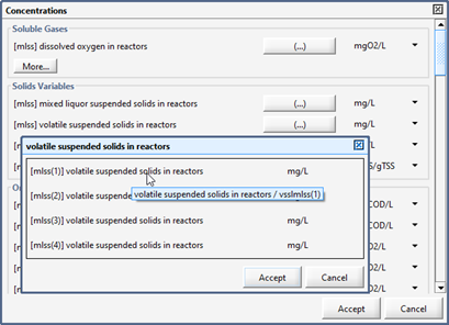
Figure 11‑6 – Viewing Cryptic Names
14. Click Accept in the Macros dialog to save the changes.
|
NOTE: This custom code is saved in a file called ‘tutorial-11.usr’ in the same directory as the layouts folder of your GPS-X V8.0 installation file directory. You can open and edit that file in an external text editor if you would prefer instead of using the GPS-X code editor. |
15. Add user-defined input variables. This is done by choosing Layout > General Data > User Files > Constants… from the main menu. This file allows you to set up the input variables on the same type of input forms as the other GPS-X variables.
16. Modify the code to read:
!MENU ITEM:!Noise Variables
!HEADER:!Noise Variables
constant mean = 0.0 !average measurement noise !gO2/(m3.d)
constant stdev = 50.0 !measurement noise standard deviation !gO2/(m3.d)
The MENU ITEM and HEADER lines set up the menus and groupings of the variables.
The lines that start with the keyword constant signify that this variable is an ACSL constant. This keyword is followed by the cryptic name, value, label and unit (with the appropriate delimiters shown above).
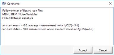
Figure 11‑7 – Adding User-Defined Inputs
17. Click Accept in the Constants dialog to save the changes. You will be prompted to reload your GPS-X layout.
|
NOTE: This custom code is saved in a file called ‘tutorial-11.con’ in the same directory as your layout. You can open and edit that file in an external text editor if you would prefer instead of using the GPS-X code editor. |
18. Save the layout and reload (close and reopen the file). This will cause GPS-X to read in your user-defined constants and create the menus associated with them. You will notice that there is now a menu item Layout > General Data > User > Input Parameters > Noise Variables.
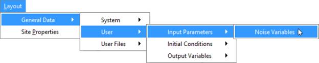
Figure 11‑8 - New User-Defined Input Parameters
19. Add user-defined output variables. This is done by choosing Layout > General Data > User Files > Output Variables from the main menu. This file allows you to set up the output variables on the same type of output forms as the other GPS-X variables.
20. Modify the code to read:
!MENU ITEM:!Uptake Variables
!HEADER:!Uptake Variables
display ourwithnoise !OUR with noise !gO2/(m3.d)
display sourone !SOUR without noise !mgO2/(gVSS.d)
display sourtwo !SOUR with noise !mgO2/(gVSS.d)
!MENU ITEM: !Noise Variables
!HEADER: !Noise Variables
display noise !measurement noise !gO2/(m3.d)
display mean !average measurement noise !gO2/(m3.d)
display stdev !measurement noise standard deviation !gO2/(m3.d)
The difference between the input variable file and this output variable file is that the keyword is ‘display’ instead of ‘constant’ and a value is not given for the output variables (because it will be calculated by the model).
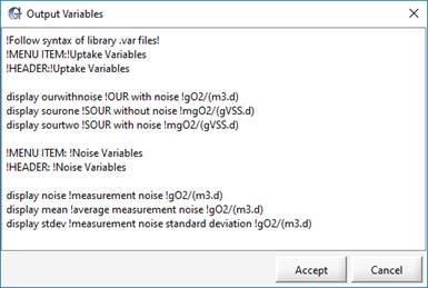
Figure 11‑9 – Adding User-Defined Outputs
21. Click Accept in the Outputs dialog to save the changes. You will be prompted to reload your GPS-X layout.
|
NOTE: This custom code is saved in a file called ‘tutorial-11.var’ in the same directory as your layout. You can open and edit that file in an external text editor if you would prefer instead of using the GPS-X code editor. |
22. Save the layout and reload. This will cause GPS-X to read in your user-defined constants and create the menus associated with them. You will notice that there are now two new menu items under Layout > General Data > User > Output Variables as displayed in Figure 11‑10.
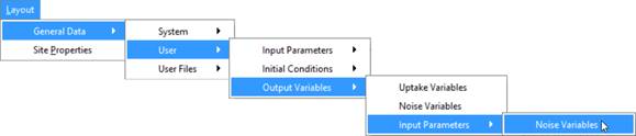
Figure 11‑10 – New User-Defined Output Parameters
23. Switch to Simulation Mode.
24. Create input controllers. Place the 2 new input variables on sliders on the controls tab. These variables can be found in Layout > General Data > User > Input Parameters > Noise Variables.
25. Change the controllers’ settings.
· For the average measurement noise, set the limits from 0 to 100.
· For the measurement noise standard deviation, set the limits from 0 to 100.
26. Create a new graph. Place the 2 new SOUR variables (SOUR without noise and Sour with noise) on a graph. These variables can be found in Layout > General Data > User > Output Variables > Uptake Variables. Set the limits from 0 to 1000.
27. Add variable to existing graph. Place the OUR with noise variable on the existing graph that we created earlier in this tutorial (i.e. with flow and actual OUR). Set the limits from 250 to 1,500.
28. Auto arrange the graphs and run a 10-day dynamic simulation with the steady-state box checked. You should produce a graph similar to Figure 11‑11.
29. Vary the noise parameters with the Input Control windows and observe the impact on the output. Try running several simulations using different settings.
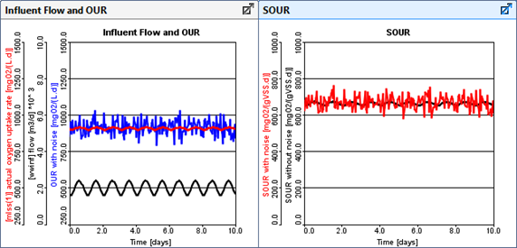
Figure 11‑11 – Simulation Results with Noise
With many of the dynamic models used in GPS-X most of the model parameters are assumed to be constant over the entire calibration period. For example, the clarifier's flocculent zone settling parameter is normally set to one specific value for the entire simulation. One reason for doing so is that it is difficult to determine or identify the changes in this parameter over time since it is difficult to measure on-line. The best the modeler can do is assume that the parameter doesn't change over the simulation period, and therefore use only one value to fit the target or measured data.
A more rigorous approach, however, might be to try to fit the measured data by varying the parameter over the simulation period. This has two advantages: a better agreement between the model and data, and an indicator of the dynamic response of the parameter. Of course, this technique assumes that the measured data is relatively free of error.
After completing this tutorial, you should be able to set up and run the dynamic parameter estimator (DPE). The GPS-X Advanced Tools module is required to complete this tutorial.
1. Load the starting point layout. We’ve already set up a layout with the appropriate data files, controllers, and output graphs. You can find it by going to File > Sample Layouts > Tutorials> Tutorial 12 (Starting Point).
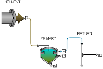
Figure 12‑1 - Layout used in Tutorial 12
2. Save the layout as a different name in your own directory. We are going to be making some changes and we’d like to leave the starting point layout as is.
3. Switch to Simulation Mode.
4. Run a 4-day dynamic simulation with the steady-state box checked.
The graph of the primary effluent TSS shows a reasonable fit with the real measured data but there is considerable room for improvement. These results are shown in Figure 12‑2.
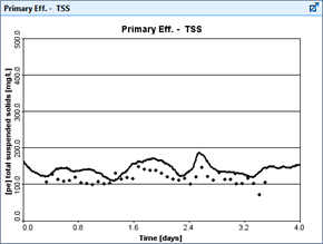
Figure 12‑2 – Primary Effluent TSS
At this point, it is desirable to improve the fit between the primary effluent TSS and the data by optimizing the flocculent zone settling parameter as it varies with time.
5. Switch to Modelling Mode.
|
|
6. Open the Optimize menu on the top toolbar and select Optimize Setup. This will display the Optimizer Setup Wizard. |
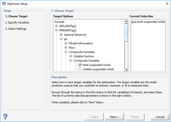
Figure 12‑3 - Optimize Setup Wizard (Target Variables)
7. Select the Target Variable. In this case, it is the total suspended solids in the reactor. It can be found under:
PRIMARY(pe) > pe > Composite Variables > Composite Variables
8. Click Next to proceed to the next stage.
9. Select the Optimize Variable. In this case, it is the flocculant zone settling parameter in the reactor. It can be found under:
PRIMARY(pe) > Settling > Double Exponential Parameters
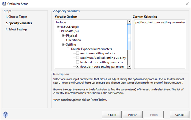
Figure 12‑4 - Optimize Setup Wizard (Optimize Variables)
10. Click Next to proceed to the next stage.
11. Specify Optimizer Settings. The last step in the process is to specify which kind of optimization we are doing. We will use Fit to Data, DPE, and Absolute Difference.
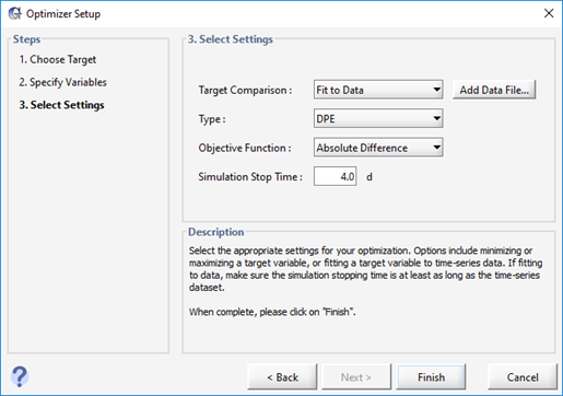
Figure 12‑5 - Optimize Setup Wizard (Optimizer Settings)
We can also use the “Add Data File…” button here to add data if needed, but we have already specified our data file so we don’t need to do it again here.
12. Click Finish to complete the set up.
13. Switch to Simulation Mode.
Note that a new input panel has been created with our optimize variable already set to the optimize type. The target variable has also been plotted on a new graph.
14. Enter Optimization Mode. Open the Optimize menu on the top toolbar and select Optimize.
15. Change the limits of the optimize variable. Edit the settings and change the min/max to 0.0001 and 0.005 respectively.
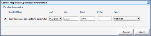
Figure 12‑6 – Optimize Parameter Limits
16. Save the layout.
17. Run the simulation. The results are shown in Figure 12‑7 and Figure 12‑8.
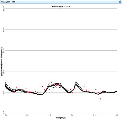
Figure 12‑7 – DPE Results
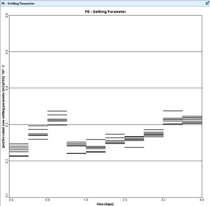
Figure 12‑8 – Flocculent Parameter
Try repeating the simulation with a shorter time window or tighter convergence criteria. These settings have been set up as input control sliders on the “DPE Settings” tab.
When developing a plant model, we may wish to not only explore what loads a plant will fail under, but the frequency with which these failures might occur. While linear analysis can tell us at which points the plant will fail, Monte Carlo analysis allows us to determine the frequency with which the plant will fail.
Monte Carlo analysis is also useful in exploring plant performance under different design assumptions. For example, when designing a plant, you need to choose a value for the autotrophic maximum specific growth rate and the alpha factors for your reactors. Neither of these values can be fully known in advance, however we can approximate the range in which these values will fall. We may know that the alpha factor for the waste water will fall somewhere between 0.4 and 0.7 and that the probability of it being any particular number inside this range is uniform. By assigning probabilities to the range of values we can use Monte Carlo analyses to not only investigate the plant’s performance over the range but the probability of the observed performance characteristics.
The purpose of this tutorial is to develop a basic understanding of Monte Carlo analysis in GPS-X. Upon completion of this tutorial you will be able to carry out Monte Carlo analysis of model variables. In this tutorial, we will be looking into how the dissolved oxygen in the tank reactor and free and ionized ammonia in the plant effluent are affected by various alpha factors and autotrophic maximum specific growth rates.
The GPS-X Advanced Tools module is required to complete this tutorial.
The Analyze module is an optional feature of GPS-X. If you have not purchased this module, contact us for pricing information.
1. Because this feature requires multiple simulations, for demonstration purposes the work will be carried out on a simple model consisting of a Wastewater Influent, a Completely-Mixed Tank, and a Rectangular Secondary Clarifier. Start a new layout.
2. Select the Comprehensive (mantis2lib) from the Library menu (if it isn’t already selected) (see Figure 13‑1)
Figure 13‑1 - Select Library
3. Create the layoutas shown in Figure 13‑2 with a codstatesinfluent model, mantis2 CSTR model and simple1dclarifier model.
4. Save the layout with the name ‘tutorial-13.
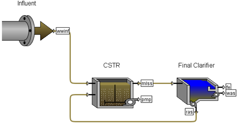
Figure 13‑2 - Tutorial 13 Layout
|
|
5. Simulate cold winter conditions. Access the Plant Wide Properties by pressing the button in the upper left corner of the drawing board. Change the liquid temperature to 10°C. |
6. Change CSTR parameters.
· Set Input Parameters > Operational > specify oxygen transfer by to Entering Airflow.
· Set the air flow into aeration tank to 15,000 m3/d.
7. Change the clarifier parameters.
· Set Input Parameters > Operational > pumped flow to 70 m3/d.
8. Save the layout.
9. Switch to Simulation Mode.
10. Create input controls. From the CSTR object, drag the following parameter to a new input control tab:
· maximum growth rate for ammonia oxidizer from Input Parameters > Kinetic (Ammonia-Oxidizing Biomass section)
· maximum growth rate for nitrite oxidizer from Input Parameters > Kinetic (Nitrite-Oxidizing Biomass section)
· alpha factor (fine bubble) from Input Parameters > Operational (Diffused Aeration section’s ‘More’ button)
11. Edit the controller settings. Open the properties window and change the maximum growth rate for ammonia oxidizer settings to:
· a min/max of 0.5 and 1.2, respectively
· the controller type to “Analyze – Monte Carlo”. Notice that a button icon appeared beside the Type box. This allows you access to the Distribution settings.
· edit the Distribution settings and change the Type to Normal, the mean to 0.9, and the standard deviation to 0.1.
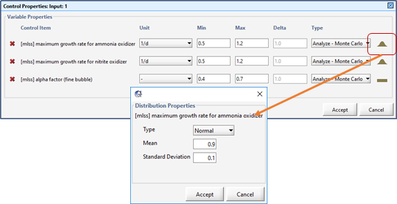
Figure 13‑3 – Monte Carlo Controller Settings
Similarly, for the maximum growth rate for nitrite oxidizer, change the min/max to 0.5 and 1.2 and change the type to “Analyze – Monte Carlo”. Also change the distribution to Normal but, in this case, change the mean to 1.0 and the standard deviation to 0.1.
This allows the two parameters to vary about the default model settings.
For the alpha factor, set the min/max to 0.4 and 0.7 and the controller type to “Analyze – Monte Carlo”. Leave the distribution as Uniform.
12. Create another input control. We will also want to vary the number of Monte Carlo runs, so we’ll create another input controller for the number of runs. That variable can be found from the main menu in:
Layout > General Data > System > Input Parameters > Simulation Tool Settings
We will now set up separate output graphs of our input (to see the input distributions that were generated) and output (which will tell us how well the plant performed).
13. Create graphs of our input variables. Note that these are the output variables representing the input parameters. You can’t drag the input parameter itself to a graph.
Create an output tab labeled “Input Distributions” and add the following parameters to their own separate graphs:
· maximum growth rate for ammonia oxidizer from the CSTR’s Output Variables > Input Parameters > Kinetic (Ammonia-Oxidizing Biomass header) menu.
· maximum growth rate for nitrite oxidizer from the CSTR’s Output Variables > Input Parameters > Kinetic (Nitrite-Oxidizing Biomass header) menu.
· alpha factor (fine bubble) from Output Variables > Input Parameters > Operational (Diffused Aeration section’s ‘More’ button, Diffused Air header) menu
14. Create graphs of our output variables.
Create an output tab labeled “Output Distribution” and add the following parameters to their own separate graphs (from the CSTR’s Output Variables > Concentrations form):
· dissolved oxygen,
· ammonia nitrogen,
· nitrite
· nitrate
15. Edit the graphs’ settings.
For all of the graphs on both tabs, change:
· the graph type to Probabilistic (Monte Carlo)
· select Autoscale for both the x and y axes
This graph type will plot a histogram of our Monte Carlo results.
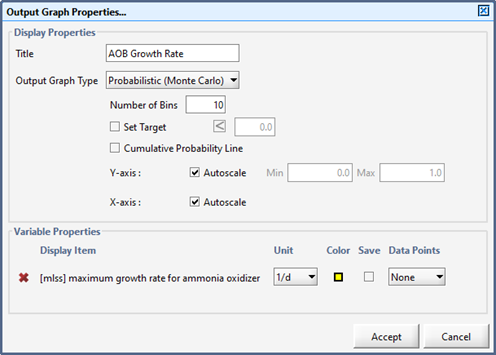
Figure 13‑4 – Monte Carlo Graph Properties
In addition, for the dissolved oxygen and ammonia nitrogen graphs, set:
· the number of bins to 20 (to see the distribution at a higher resolution)
· the target values to < 3.0 for ammonia nitrogen and >2.0 for dissolved oxygen (you can change the sign of the <, > symbol by left-clicking on the icon)
16. Save the layout.
|
|
17. Select the Monte Carlo analysis type. Click the little arrow beside the Analyze button on the main toolbar (or access it through the main menu’s Tools > Analyze) and select “Monte Carlo”. |
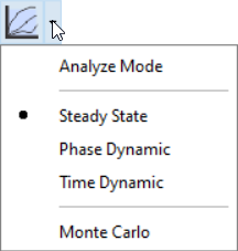
Figure 13‑5 - Selecting Analysis Type
Switch to Analyze Mode. Click the Analyze button on the main toolbar (or access the Analyze Mode checkbox through the main menu’s Tools > Analyze) to turn on the analyzer.
The status bar at the bottom right of the main window will indicate that you are in Analyze Mode.
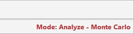
Figure 13‑6 - Status Bar showing “Analyze – Monte Carlo” Mode
18. Run the simulation. The simulations will run one after another, while collecting the output of the model for post-simulation analysis. You can follow the progress of the simulations on the Input tab, as the red indicator on the three input parameters progresses through the required simulations (1000 of them, by default). Note that it may take several minutes for the simulations to complete, depending on the speed of your computer.
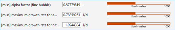
Figure 13‑7 - Tracking the Progression of the Simulations
When the simulations are completed you should see the distribution of input parameters for the alpha constant and the two growth rates. The growth rates should follow a normal distribution, whereas the alpha factor should have a uniform (flat) distribution. Note that the distribution of actual values used may not quite fit the expected distribution shape. This is due to only running 1000 simulations – it would be more representative of the desired distribution with larger numbers of simulations.
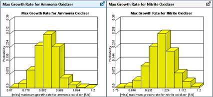
Figure 13‑8 – Input Parameter Distributions
The graphs on the Output Distributions tab shows the performance of the plant under the varying model input. The effluent ammonia graph illustrates that the plant is nitrifying most of the time. The target line shows that the plant effluent ammonia is equal to or less than the target 3.0 mgN/L in 88.6% of the simulations. Note that in the Monte Carlo analysis you may receive slightly different solutions but the % value recorded on the graph should be within the range of 85% to 90%.
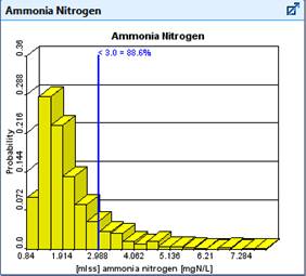
Figure 13‑9 – Output Distribution Results
showing Target
19. Rerun the simulation. However, this time use a larger aeration capacity. Create a new scenario, and try increasing the aeration tank volume and/or the airflow to the system. How much larger does it have to be to have 95% of the simulations with effluent ammonia at 3.0 mgN/L or less?
No software package can be created generally enough such that it can automatically handle every user’s exact display and interfacing needs. To offer the user with the greatest degree of customizability, Python has been fully integrated into GPS-X. Through integrating Python in GPS-X, advanced users have the ability to customize how they use GPS-X, from creating unique visuals to the automation of data collection. The use of this feature requires the user to be familiar with the Python programming language. Some basics of the Python language will be highlighted throughout the following tutorials, but they are not meant as a comprehensive guide for using Python.
In this tutorial, you will begin by familiarizing yourself with how Python is implemented in GPS-X and how Python can be customized. You will then learn how Python can be used to directly manipulate variables in a GPS-X simulation.
The GPS-X Advanced Tools module is required to complete this tutorial.
After completing this tutorial, you should be able to create Python scripts that can run and manipulate GPS-X simulations.
1. Open the Layout created in Tutorial 1 and save it as `tutorial-14’ .

Figure 14‑1 – Tutorial 14 Layout
2. Switch to Simulation Mode, if it is not already selected.
3. Open Python Script Manager. Python’s functionality within GPS-X is managed through the Python Script Manager.
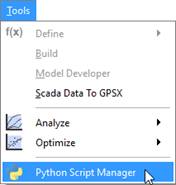
Figure 14‑2 – Accessing the Python Script Manager
4. Create a New Script. Pressing the new button will prompt you to create a new Python script. By default, the script will be saved in the same directory as the layout with the same name as the layout. Save the script using the default settings.
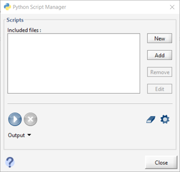
Figure 14‑3 - Creating a New Python Script in GPS-X
5. Edit the Script. With “tutorial-14.py” selected, which is indicated by the file name being highlighted in a dark blue color, press the Edit button. By default, this will open the Python script in Notepad using Python version 3.7.
|
|
These default settings can be changed by pressing the Python Settings button. GPS-X comes with versions 2.7 and 3.7 of Python in the install and you can easily toggle between these versions from this menu. You can also specify other versions of Python on your machine that you would like GPS-X to use by selecting the other option in the Python Settings menu and specifying both the version number and the pathway of the Python instance. The default text editor can also be changed from this menu if desired. |
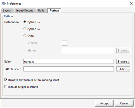
Figure 14‑4 - Python Settings Menu
6. Every Python script generated by GPS-X will be initially populated with 4 GPS-X recognized functions. An unedited Python Script generated by GPS-X can be seen in Figure 14‑5. The functions that GPS-X predefines in the script are:
i. start – This function is called a single time at the start of a simulation.
ii. cint – This function is called at each communication interval that occurs in the simulation.
iii. eor - This function is called a single time at the end of a GPS-X simulation.
iv. runSim – This function starts the GPS-X simulation within the Python script. A simulation will begin each time this function is called within the script.
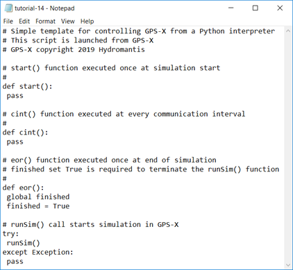
Figure 14‑5 – Python Script Generated by GPS-X
7. As a means to familiarize yourself with how the Python interfaces within GPS-X, we will begin with a Hello World example:
In the start() function, replace the pass command with:
print(“Hello”)
In the cint() function, replace the pass command with:
print(“ “)
Finally, in the eor() function, add the following line after the finished = True statement:
print(“World”)
The updated script can be seen in Figure 14‑6.
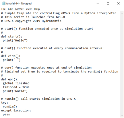
Figure 14‑6 - Sample Python Script
8. Save the Script. After making changes to the script in Notepad, the file must be saved in Notepad before it can be run in GPS-X. This is done by selecting File > Save from the main toolbar in Notepad.
|
|
9. Run the Script. Return to the Python Script Manager. The “tutorial-14.py” script will currently be the only script available in the Python Script Manager, so it will be selected by default. Press the Run Script button to run the selected Python script within GPS-X. The Python Script manager will then run your Python script. |
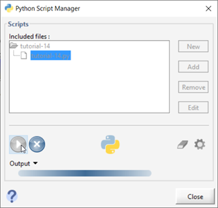
Figure 14‑7 - The Python Script Manager Running a Python Script
10. The results of the script appear in the Output pane of the Python Script Manager, which can be accessed by pressing the Output button. The results of the simulation can be seen in Figure 14‑8. “Hello” is the first output in the output pane and it appears only a single time. The output “Hello” appears first because the start function is called immediately when a simulation begins. The start function is not called again during the simulation, so “Hello” will only appears a single time. Likewise, “World” only appears a single time at the end of the output due to the eor function only being called once at the end of the simulation.
In the output, it can be seen that the cint function is called twice during the simulation, creating the two blank lines between “Hello” and “World”. The cint function is called at every communication interval in the simulation which includes both the initiation of the simulation after the start function (t = 0.0) and when the simulation terminates prior to calling the eor function. Due to the stop time in this simulation being set to 0.0 days, cint will only be called at the initiation and termination of the Python script, causing two instances of “ “ to appear in the output.
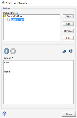
Figure 14‑8 - Results of Running the Python Script
Now that a you have an understanding of how Python scripts are used to communicate with GPS-X, we will move to an example that is more focused on how we can use Python to manipulate the variables within GPS-X.
11. Save a New Script. We have created a Python script for you to use during this portion of the tutorial. Locate and open the “tutorial-14-COD-Manipulation.py” Python script file located in the following subdirectory of the GPS-X instillation directory:
\layouts\08tutorials\
Save the script in the directory where the GPS-X file is currently saved.
12. Open the Python Script Manager.
13. Add the Script. When using an existing Python script, it must be added to the Python Script Manager before you can run it in GPS-X. Press the Add button.
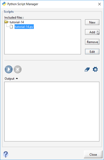
Figure 14‑9 - Adding an Existing Script to the Python Script Manager
Pressing Add will open the current working directory and show all Python files currently saved in the directory. Select the “tutorial-14-COD-Manipulation.py” file and Open it to add it to the Python Script Manager.
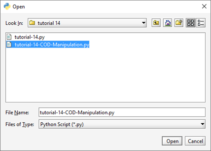
Figure 14‑10 - Adding the tutorial-14-COD-Manipulation File to the Python Script Manager
14. Edit the Script. Select the “tutorial-14-COD-Manipulation.py” script and press Edit. This will open the script in Notepad. We will now examine the important components of the Python script:
The start function can be seen in Figure 14‑11. The start function in this script is used to display the initial value of some GPS-X variables of interest. Python is then used to directly change the value of these variables in GPS-X. This is done using predefined commands that are recognized by GPS-X. The GPS-X recognized commands in the start function include:
· gpsx.getValue. This function is used to get the value currently assigned to a variable in GPS-X for manipulation in Python. To use the getValue function, you must enter the cryptic name of the of the GPS-X variable in the parenthesis as a string.
· gpsx.setValue. This function is used to assign new values to GPS-X variables directly through Python. To use this function, you must first enter the cryptic name of the GPS-X variable in the parenthesis as a string. The new value you would like to assign to the variable is then entered. Ensure that the appropriate Python variable type is used in this function.
Note: If you would like to toggle an ON/OFF switch in GPS-X, you must use the gpsx.setValue and assign it a value of 0.0 for OFF and a value of 1.0 for ON.
· gpsx.setTstop. This function is used to change the stop time of the current simulation. To use this function, simply enter the new stop time you would like in the parenthesis
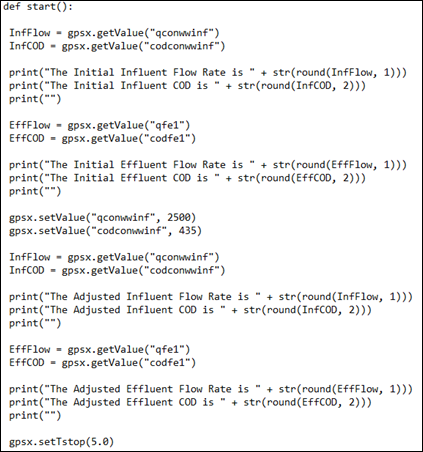
Figure 14‑11 - The Start Function in the tutorial-14-COD-Manipulation Python Script
The cint function can be seen in Figure 14‑12. Using the gpsx.getValue function, the cint function obtains the final values of our variables of interest.
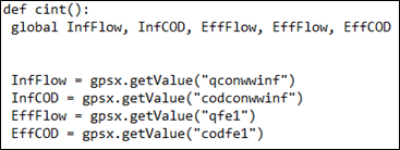
Figure 14‑12 - The cint Function in the tutorial-14-COD-Manipulation Python Script
The eor function can be seen in Figure 14‑13. This function is simply used to format the data collected in the cint function.
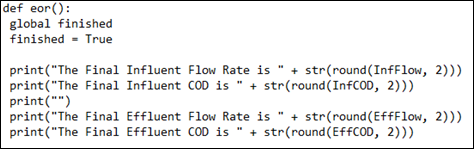
Figure 14‑13 - The eor Function in the tutorial-14-COD-Manipulation Python Script
15. Save the Script.
16. Run the Script. The simulation output can be seen in Figure 14‑14. From the output, it is important to note that changing the value of a GPS-X variable with Python will not have an immediate effect on the other variables in GPS-X. This is illustrated when looking at the Adjusted influent and effluent variables in the output. Well Python changes the influent variables, the effluent variables remain unchanged. The effluent variables will not be calculated until the simulation resumes. You can use Python to access the newly calculated effluent variable values at the next communication interval.
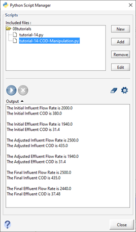
Figure 14‑14 - Output of the tutorial-14-COD-Manipulation Python Script
The power of using the Python programming language alongside GPS-X comes from Python’s active community of users making open source libraries that preform a variety of functions in Python. To use these libraries, you are required to install them in the directory where you are running Python from. This tutorial will focus on the instillation of Python in a Windows environment assuming an internet connection is available for your machine.
17. Open the Command Window. The command window can be opened by going to the start menu and typing ‘cmd’. Hit the Enter key.
18. Access the Directory. You need to access the directory where GPS-X has been installed on your computer. Once you have found the GPS-X directory, you will need to create a path to it in the command window.
If you are using Python version 3.7, open the folder named python37 in the GPS-X instillation directory. Copy the address of the directory by right clicking on the file explorer address bar and selecting Copy address. The address will end in:
GPS-X80\python37
If you are using Python version 2.7, open the folder named python in the GPS-X instillation directory. Copy the address of the directory by right clicking on the file explorer address bar and selecting Copy address. The address will end in:
GPS-X80\python
In the command window, enter cd and paste the copied address. Hit Enter to make this the active directory.
cd <Paste address here>
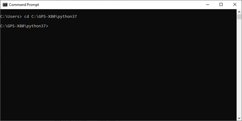
Figure 14‑15 - Accessing the GPS-X Python directory
19. Update pip. pip is a package installer included in the base Python instillation that is used to install libraries in Python. First ensure pip is fully updated by typing:
python -m pip install --upgrade pip
Press the enter key. Using an Internet connection, pip will search to see if any updates are available for the pip library. If updates are available, pip will update itself and any out of date dependencies.
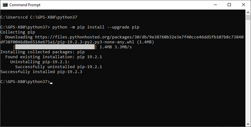
Figure 14‑16 - Updating the Python pip Package Manager
20. Install matplotlib. We will now be installing matplotlib, a library that is used for plotting data within Python. To install matplotlib, type the following into the command window and hit Enter:
python -m pip install matplotlib
pip will automatically install matplotlib and its dependencies in the specified directory.
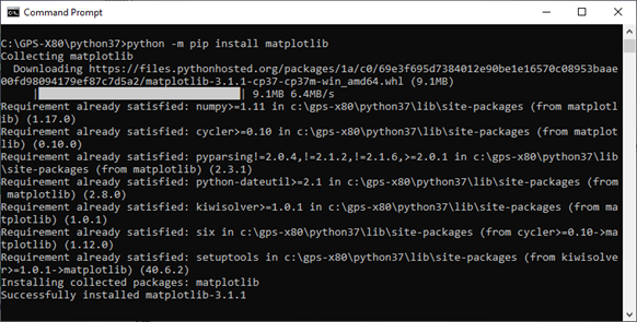
Figure 14‑17 - pip Installing matplotlib
21. Check the Install. Any libraries that you have installed to your version of Python can be seen in your GPS-X download directory. If you are using Python 3.7 go to:
GPS-X80>python37>Lib>site-packages
If you are using Python 2.7 go to:
GPS-X80>python>Lib>site-packages
When building a model, it is often easy to overlook that many variables in the system may exhibit random behaviour. Additionally, if it is recognized that some variables, such as storm frequency and severity, historic data may be unavailable and creating data for the simulation may introduce an input bias to the system. By using Python, we can introduce truly unique data to the system and visualize how it will react.
By using random inputs, you can see how your wastewater treatment plant will react under unpredictable operating conditions. For example, when designing a plant, data may be available that details the influent that the plant can expect, but this data often omits random and unpredictable events such as storms that will impact your influent flow. Using Python’s random number generator, we will create a simulation to visualize the effects of storm frequency and severity on the influent flow rate to a plant and how this flow rate can be controlled.
The GPS-X Advanced Tools module is required to complete this tutorial.
Upon completion of this tutorial, you will have an understanding of how Python’s random number generator can be used to generate random events in GPS-X and visualize the impact they on the operation of your plant.
1. Create a new layout consisting of:
· A wastewater influent object,
· a stormwater runoff (Influent tab)
· a 2-flow combiner,
· a plug-flow tank,
· a circular secondary clarifier
· a wastewater outfall
Use the mantis2lib library and the default model selections (the codstates influent model, the mantis2 plug flow tank model and the simple1d circular clarifier model).
Connect the unit processes and add the labels displayed in Figure 15‑1.
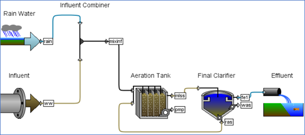
Figure 15‑1 - Tutorial 15 Layout
2. Save the layout as ‘tutorial-15’.
3. Enter Simulation Mode.
4. Create an output plot for the flow leaving the Influent Combiner as described in Tutorial 2 (Right click the 2-flow combiner object Output Variables > Flow). Set the plot to autoscale.
5. Open the Existing Python Script. We have included a pre-written Python script for creating a random event. Locate and open the tutorial-15-Random.py Python script in the following subdirectory of the GPS-X installation:
\layouts\08tutorials\
6. Save the Python Script. Save the Python script in the same directory as the layout file.
7. Add the Python Script to the Layout. In the Python Script Manager press the Add button and select the script. Press Open.
8. Edit the Python Script. Press the Edit button to open the script in Notepad. The script has been broken into 2 sections:
· User Inputs:
The User Inputs section currently contains a list variable that corresponds to the rain fall depths that the Stormwater Runoff object can generate in mm/hr. It also contains a variable that will represent the user defined communication interval and stop time.
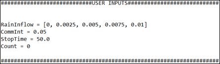
Figure 15‑2 - The User Inputs Section of the Python Script
· Functions:
The Functions section of the script contains the four functions that are automatically generated by GPS-X when creating a new Python script. In the Start function, a new pre-defined GPS-X recognized command, gpsx.setCint is introduced. This command allows you to change the communication interval used in the GPS-X simulation directly within Python. To use the gpsx.setCint command, enter the desired communication interval in the parenthesis.
The randomness in this script is introduced in the cint function. In the cint function, Python’s random library is used to generate random integer numbers. Using conditional formatting, these random integers are then used to assign a value to the rainfall depths variable in the Stormwater Runoff object, creating random behaviour in the simulation.
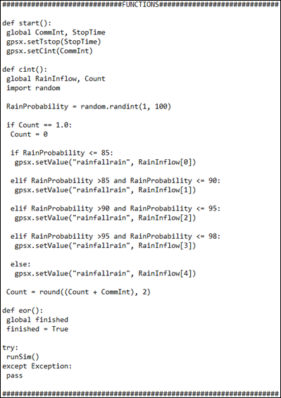
Figure 15‑3 - The Functions Section of the Python Script
9. Save the Python Script.
10. Run the Script. Press the Run button in the Python Script Manager. A sample output graph can be seen in Figure 15‑4. Note: Your graph will appear different than what is seen here due to the randomness introduced by the Python script.
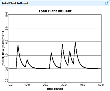
Figure 15‑4 - Output Graph of the Random Rain Event
With the introduction of a random rainfall event, the total influent to the plant may reach values that exceed the maximum capacity of the treatment equipment. To accommodate this, we will use Python to simulate a bypass weir.
11. Enter Modelling Mode.
12. Add the following objects:
· A Control Splitter (This will act as our bypass weir),
· a 2-flow Combiner
Adjust the unit connections and stream labels as seen in Figure 15‑5.
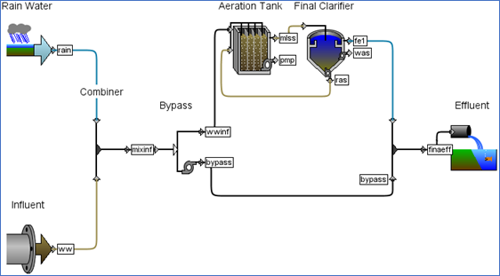
Figure 15‑5 - Tutorial 15 Layout with a Bypass Introduced
13. Switch to Simulation Mode
14. Create an Output plot with the following variables:
· Total Influent can be found in the Influent Combiner Output Variables > Flow
· The Aerator flow can be found by by right clicking the wwinf connection point on the Control Splitter Output Variables > Flow
· The Bypass flow can be found by by right clicking the bypass connection point on the Control Splitter Output Variables > Flow
15. Open the Python Script Manager
16. Edit the Python Script. Select the “tutorial-15-Random.py” Python script and hit the Edit button on the Python Script Manager.
17. Save the Script. We will be modifying the “tutorial-15-Random.py” Python script in our new scenario. To avoid changing the script used in the previous section, go to File > Save As. In the Save As window change the Save as type to All Files and save the script with a new name ending in .py extension (eg. “tutorial-15-Bypass.py”)
18. We will need to make following changes to the Python script:
· Add the following to the User Input Section:
MaxAeratorFlow = 4000
This value represents the maximum allowable flow rate that the Aerator can handle.
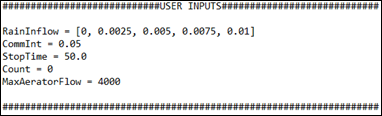
Figure 15‑6 - Changes to the User Inputs Section in the Bypass Python Script
· Add the following to the global variables defined at the start of the cint section:
MaxAeratorFlow
· Add the following to the end of the cint function:
Inflow = gpsx.getValue('qmixinf')
if Inflow > MaxAeratorFlow:
gpsx.setValue('qconbypass', (Inflow - MaxAeratorFlow))
else:
gpsx.setValue('qconbypass', 0.0)
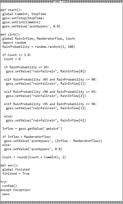
Figure 15‑7 - Changes to the Functions Section in the Bypass Python Script
This block finds the total influent that is entering the plant from both influent objects and determines if it is greater than what the Aerator can handle. If the influent flow rate is greater than the maximum aerator flow rate, the excess is bypassed.
19. Save the Script.
20. Run the Script. A sample output can be seen in Figure 15‑8. Note: your output will appear different due to the randomness in this script.
Notice that by controlling the bypass this way, any flow that would exceed the maximum allowable aerator influent of 4,000 m3/d is instantaneously bypassed and the influent limit is never exceeded.
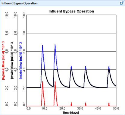
Figure 15‑8 - Output of the "tutorial-15-Bypass" Python Script
When running a GPS-X simulation, changes caused by control loops happen instantaneously, but this assumption does not always translate directly to the real world as input delays and equipment start up times may cause a discrepancy between the detection of an event and when it is corrected for. We will now look at how we can use Python to delay the time it takes for the model to address a deviation from setpoint.
21. Open the Existing Python Script. We have included a Python script that has already been written to delay the bypasses ability to control the influent. Locate and open the tutorial-15-Delay.py Python script in the following subdirectory of the GPS-X installation directory:
\layouts\08tutorials\
22. Save the Python Script in the active directory
23. Open the Python Script Manger
24. Add the Script to the Python Script Manager
25. Edit the Script. This Python script is built from the “tutorial-15-Bypass.py” Python script. We will now discuss the changes made from that Python script:
· Influent: A list variable called Influent has been added to the start function. This variable is used in the cint function to collect the total influent flow at every communication interval.
· Count: A variable called count has been added to the start function. This variable is used to track the number of communication intervals that have occurred. The communication interval time has been reduced in this Python script, so the count variable tracks the communication intervals to ensure the random event still occurs on the communication interval that corresponds to 1 day being elapsed.
· Bypass Control: The bypass control from the previous Python script has been modified and now compares the total influent flow that occurred 5 confidence intervals prior to the maximum allowable flow rate to the aerator. This introduces a delay of 5 communication intervals to the bypasses ability to control a deviation in the influent flow rate.
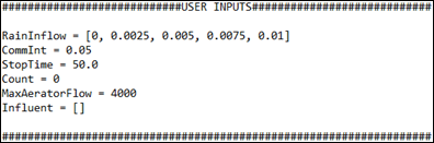
Figure 15‑9 - Changes to the User Inputs Section of the Delayed Bypass Python Script
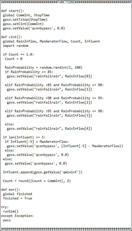
Figure 15‑10 - Changes to the Functions Section of the Delayed Bypass Python Script
26. Save the Script
27. Run the Script. A sample output can be seen in Figure 15‑11. Note: your output will appear different due to the randomness in this script.
Notice that when the Aerator influent limit is exceeded, the bypass does not immediately activate, and excess influent enters the Aerator. It can also be noted that when the bypass is activated, that the amount bypassed exceeds what is actually required to meet the maximum influent allowed to enter the aerator.
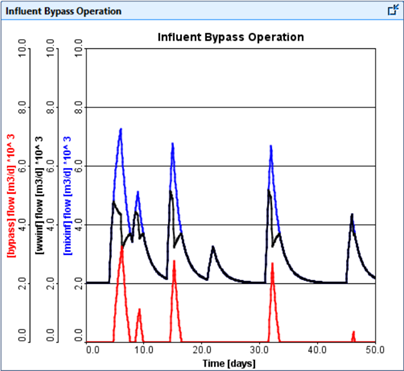
Figure 15‑11 - Output of the "tutorial-15-Delay" Python Script
When creating a new model, it is common to preform a sensitivity analysis to analyze the effects that uncertainty in your parameters will have on the model. While visualizing the effects of changing a single parameter may offer the user a way to test the validity of a given model, it is often difficult to visualize the effects the effect that simultaneously changing multiple parameters will have on the model.
By systematically altering the parameters used in a given system, you can develop a detailed understanding of how the variables in your model interact with each other. Through the use of Python, the analysis process in GPS-X can be simplified and you can create detailed sensitivity maps to visualize the relationship between variables in your system.
In this tutorial, the sensitivity of a plant’s effluent ammonia will be examined using two different methods. First, we will look at the sensitivity of effluent ammonia to simultaneous changes to both liquid temperature and the secondary clarifier’s wastage flow rate by producing a 3-Dimensional sensitivity map. We will then explore how various sets of operating conditions can be compared to each other directly on a 2-Dimensional plot using scenarios in GPS-X.
The GPS-X Advanced Tools module is required to complete this tutorial.
The purpose of this tutorial is to see how Python can be used to maximize the information you extract from GPS-X. By the end of this tutorial, you can use Python to create detailed sensitivity analysis in GPS-X.
Plots in this section will be created using the matplotlib library in Python which must first be installed into Python, as described in Tutorial 14. The plots will be displayed using the Pillow (referred to as PIL in python) library which also must be installed.
We will now look at how Python can be used to model the sensitivity of an output variable to two simultaneously manipulated inputs. Ensure matplotlib and Pillow have been install to the instance of Python you are using as described in Tutorial 14 before proceeding with this Tutorial.
1. Open the layout created in Tutorial 1 and save it as ‘tutorial-16’.

Figure 16‑1 - Tutorial 16 Layout
2. Switch to Simulation Mode if not already there.
3. Open the Existing Python Script. We have included a Python script that has already been written to perform the sensitivity analysis. Locate and open the ‘tutorial-16-3D.py’Python script found in the following subdirectory of the GPS-X installation:
\layouts\08tutorials\
4. Save the Python Script. Save the script in the current working directory.
5. Open the Python Script Manager. The Python Script Manager can be accessed by through Tools > Python Script Manager on the main toolbar.
6. Add the Script to the Python Script Manager. Press the Add button and select tutorial-16-3D.py from the menu. Press Open to add it to the Python Script Manager.
7. Edit the Script. Press the Edit button to open the Python script in Notepad.
The script is broken into 4 major sections:
· User Inputs:
The user inputs section is where the user can define the range of values they would like to include in the sensitivity analysis. The user can specify upper and lower bounds for both the liquid temperature and the Secondary Clarifier wastage flowrate.
The user can also specify the number of points they would like to use in the sensitivity analysis. The range between the minimum and maximum values assigned to each variable will be split into this many equally spaced points. A simulation will be run at each of these conditions.
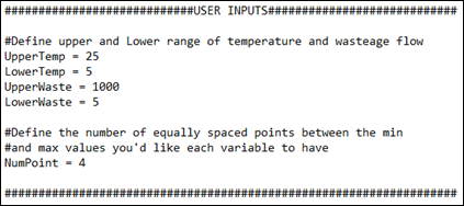
Figure 16‑2 - The User Inputs Section of the Python Script
· Functions:
The functions defined by GPS-X when creating a new Python script are used to manipulate variable values in GPS-X. An additional function, GpsxFn, has been added to this section. This is a user defined function. It is used to set the values for Temperature and Wastage Flow to be used in the current.
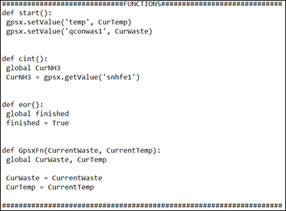
Figure 16‑3 - The Function Section of the Python Script
· Data Collection:
This section of the script creates the range of values to be looked at using Python’s numpy library. Using numpy, a coordinate matrix is constructed for each of the variables. The values in the matrices are equally spaced between the minimum and maximum values defined in the user inputs section. Each of these coordinates is then feed into the GPS-X simulation to determine the effluent Ammonia concentration under these operating conditions. These effluent concentrations are extracted from GPS-X and recorded in a results matrix.
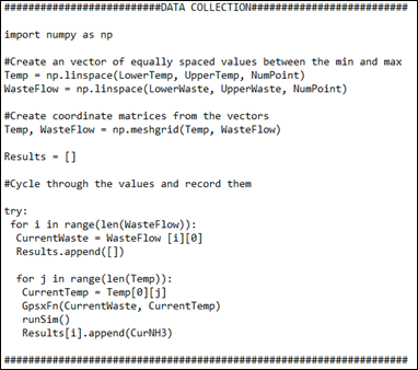
Figure 16‑4 - The Data Collection Section of the Python Script
· Plotting:
This section uses Python’s matplotlib library to create a 3-D plot of the data collected in the previous section of the Python script. The plot will be saved as a .png file in the same directory as the layout file at the end of the Python Script. Pillow is then used to open this PNG file prior to terminating the script.
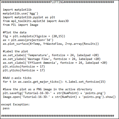
Figure 16‑5 - The Plotting Section of the Python Script
8. Save the Python Script.
9. Run the Python Script. Press the Run Script button on the Python Script Manager window.
10. View the Results. The plot produced by the script is saved as a .png file in the directory where the layout file is saved. Open the directory where you have saved the layout file and locate the PNG file named “Tutorial-16-3D-4points.png”. Open the PNG file to view the results of the sensitivity analysis
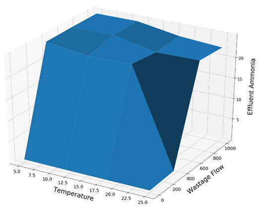
Figure 16‑6 - Sensitivity of Effluent Ammonia to Liquid Temperature and Wastage Flow
11. Edit the Python Script. In the User Inputs section of the Python script, make the following changes:
· Increase the LowerTemp value to 10 °C (this will decrease the temperature range being looked at, as little change is observed between 5 °C and 10 °C).
· Increase the NumPoint value to 10 (This will increase the resolution of the of the data as more points are being sampled allowing you to better visualize trends). Note: The increased number of points will require more simulations and will take longer to run than the previous script.
12. Save the Python Script.
13. Run the Python Script.
14. View the Results. Open the new PNG figure found in the active directory called “Tutorial-16-3D-10points.png”. Notice that the resolution of the plot has increased due to the increased number of sample points being used.
Note: When deciding on the number of points to use in a sensitivity analysis, keep in mind that the number of simulations required does not grow linearly with the number of points. A large number of points to be examined can lead to long wait times depending on the speed of your computer and the complexity of your layout.
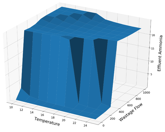
Figure 16‑7 - Sensitivity of Effluent Ammonia to Liquid Temperature and Wastage Flow with an Increased Number of Sample Points
We will now examine how we can visualize the effects of changing multiple variables in a simulation at once by using both GPS-X’s Scenario functionality and the matplotlib Python Library
15. Create Two New Scenarios. Information on creating new scenarios can be found in Tutorial 3. Create the two new scenarios with the following specifications:
· High Flow:
o Derived new scenario from: Base Model
o Change Influent Flow Rate, found under Influent > Flow > Flow Data, to 4,000 m3/day
o Change Aerator maximum volume, found under Aeration Tank > Input Parameters > Physical, to 1,500 m3
· Low Flow:
o Derived new scenario from: Base Model
o Change Influent Flow Rate, found under Influent > Flow > Data, to 500m3/day
o Change Aerator volume, found under Aeration Tank > Input Parameters > Physical, to 750 m3
16. Open the Existing Python Script. We have included a pre-written Python script that will perform a 2-Dimensional sensitivity analysis. Locate and open the tutorial-16-2D.py Python script found in the following subdirectory of the GPS-X installation directory:
\layouts\08tutorials\
17. Edit the Script. Press the Edit button to open the Python script in Notepad. The script is setup using the same 4 sections as the previous script. We will now walkthrough what each section does:
· User Inputs:
The user must define the temperature range they are interested in viewing and the number of equally spaced points they would like this range to be broken into. You can also specify the target effluent ammonia concentration, which will be superimposed on our output graph.
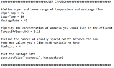
Figure 16‑8 - The User Input Section of the Python Script
· Functions:
The functions defined by GPS-X when creating a new Python script are used to manipulate variable values in GPS-X. A user defined function GpsxFn is also included to manage the scenario and temperature to be used in the current simulation. In the GpsxFn function, a new GPS-X recognized command, gpsx.setScenario, is introduced. This command allows you to select which scenario will be active during the GPS-X simulation by including the name of the scenario as a string in the parenthesis.
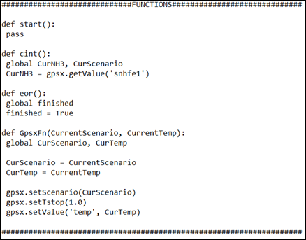
Figure 16‑9 - The Function Section of the Python Script
· Data Collection:
The temperature range to be examined is converted to a vector of equally spaced points in this section. This vector is then cycled through and each temperature in the vector is applied to each GPS-X scenario being analyzed. The effluent ammonia in each scenario is extracted from GPS-X and recorded to a list of results in Python.
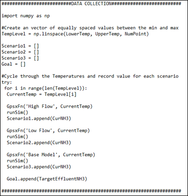
Figure 16‑10 - The Data Collection Section of the Python Script
· Plotting:
The results of the simulations are plotted on a single axis. A line representing the target effluent ammonia concentration is superimposed on the graph. The graph is then saved as a PNG file in the same directory the layout file is saved in with the name “Tutorial-16-2D-4points.png. Pillow will open this PNG at the end of the simulation.
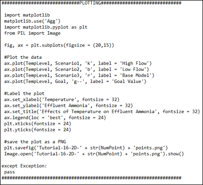
Figure 16‑11 - The Plotting Section of the Python Script
18. Save the Script.
19. Run the Python Script. Press the Run Script button on the Python Script Manager window.
20. View the Results. The plot produced by the script is saved as a .png file in the directory where the layout file is saved. Open the directory where you have saved the layout file and locate the file named “Tutorial-16-2D-4points.png”. Open the image file to view the results of the script.
From the results, we can see how the three different scenarios compare to each other. The Low Flow and Base Model scenarios are similar for all temperatures, but they both have a lower effluent ammonia concentration than the High Flow scenario at low temperatures. Using the superimposed goal line, we can also determine that the Low Flow and Base Model scenarios have an acceptable effluent ammonia concentration at a liquid temperature of ~ 16 °C while the High Flow scenario has an acceptable effluent ammonia concentration at a liquid temperature of ~ 19 °C.
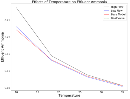
Figure 16‑12 - Effects of Liquid Temperature on Effluent Ammonia
21. Rerun the Script with new conditions. Increase the number of the number of points to be analyzed in the temperature range to 10. Increase the influent flow rate in the High Flow scenario to 5,000 m3/d.
The integration of Python in GPS-X allows you to customize how you use GPS-X and well there is a wealth of open source libraries available for Python, there may not always be a library available that meets your needs. To offer additional functionality to Python in GPS-X, the ability to add Java JAR files has been included. This will allow you to easily access JAR files to offer additional tools to customize your GPS-X experience.
The GPS-X Advanced Tools module is required to complete this tutorial.
The purpose of this tutorial is to develop an understanding of how Python can be used to access Java JAR files within GPS-X. In this tutorial, we will look at how JAR files can be added to GPS-X and then we will use these JAR files with the Java Virtual Machine to dynamically visualize how steady state operating conditions affect a simulation.
To use Java with Python in GPS-X, you must first provide GPS-X with a pathway to the JAR files that you would like to use. In this tutorial we will be using JAR files from JFreeChart, an open-source Java framework that is used for generating a variety of interactive charts.
1. Open a blank GPS-X layout.
2. Access the JAR files. We have included a folder containing the JAR files that you will need for this tutorial. Locate the folder “tutorial-17-JARS” in the following subdirectory of the GPS-X installation:
\layouts\08tutorials\
3. Copy the folder and paste it into your current working directory.
4. Open the Python Preferences. The Python preference menu can be opened by going View > Preferences on the main toolbar. Open the Python tab.
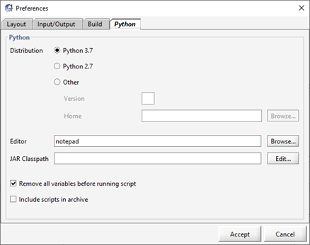
Figure 17‑1 - The Python Preferences Menu
5. Edit the JAR Classpath. Press the Edit… button next the JAR Classpath entry field to open the JAR Classpath Manager.
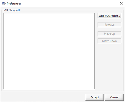
Figure 17‑2 - JAR Classpath Manager
6. Add the JAR Classpath. Press the Add JAR/Folder… button to open directory. Locate the tutorial-17-JARS folder you had previously copied and open it. Press the Add JAR/Folder button to add the entire folder to the JAR Classpath. Note that you can add single JARs using this method as well by selecting the desired JAR and then pressing the Add JAR/Folder button.
7. Accept the JAR Classpath. Press the Accept button on the JAR Classpath Manager to return to the Python preferences manager.
8. Accept the new Python Settings. Press Accept on the Python preferences screen and you will be prompted to restart GPS-X for the new changes to take effect. Press OK to accept the changes to the Python preferences and close GPS-X.
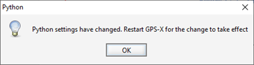
Figure 17‑3 - GPS-X Prompt to restart Python for the New Preferences to take Effect
9. Reopen GPS-X and open the layout created in Tutorial 1. Save the layout as ‘tutorial-17’.
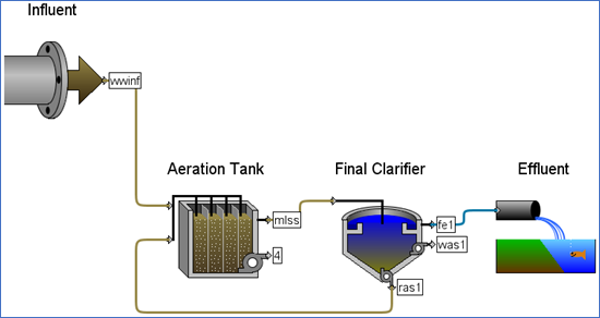
Figure 17‑4 - Layout used in Tutorial 17
10. Make the following changes to the layout:
· Change the Influent Flow Type, which can be found under Influent > Flow > Flow Type to Sinusoidal
· Change the Influent Flow Rate which can be found under Influent > Flow > Data, to 3,000 m3/day
11. Switch to Simulation Mode.
12. Save the Layout.
13. A Python script has already been created for use in this tutorial. Locate and open the Python script called ‘tutorial-17.py’. The Python script can be found in the following directory:
\layouts\08tutorials\
14. Save the Python Script. Save the script in the current working directory.
15. Add the Script to GPS-X. Open the Python Script Manager in GPS-X and add the Python script to GPS-X.
16. Edit the Script. Press the Edit button to open the script in Notepad. This script is broken into two primary sections Functions and Plotting. We will now discuss what the script is doing:
The Function section contains the standard GPS-X functions that are included when GPS-X creates a new script. The cint() function is used to collect data at every communication interval. An additional user defined function, createDialPlot, has also been added to this section. This function is used to create and format a Dial plot in the Java Virtual Machine.
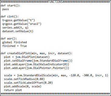
Figure 17‑5 - Functions Section of the Non-Steady State Test Python Script
The Plotting section of the script runs the simulation and creates a JPanel that the Dial plot and a XY line chart will be added to. The Dial Plot is used to track the time that has been elapsed in the simulation well the XY Line Chart tracks changes in the value of the output variable.
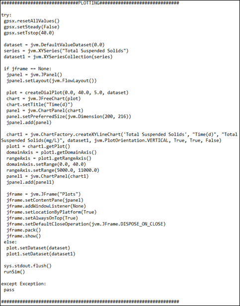
Figure 17‑6 - Plotting Section of the Non-Steady State Test Python Script
Two new GPS-X recognized Python commands are introduced in this section:
· gpsx.resetAllValues. This command is used to reset the value of all the variables back to their value when initially entering Simulation Mode. No input is required for this command
· gpsx.setSteady. This function allows you to toggle the steady state setting in GPS-X through Python. To set steady state on, type True in the parenthesis. To turn steady state off, type False in the parenthesis
17. Save the Script.
18. Run the Script. Press the Run Script button with the script highlighted.
19. By viewing the plot produced at the end of the simulation, as seen in Figure 17‑7, it can be noted that the total suspended solids in the secondary clarifiers recycle stream is initially very high and unpredictable. As the simulation continues to run, the level of total suspended solids reflects the sinusoidal influent pattern. After approximately 30 days, the output exhibits a constant upper and lower limit of total suspended solids in the recycle stream as a function of the influent flow. This is representative of the system reaching steady state.
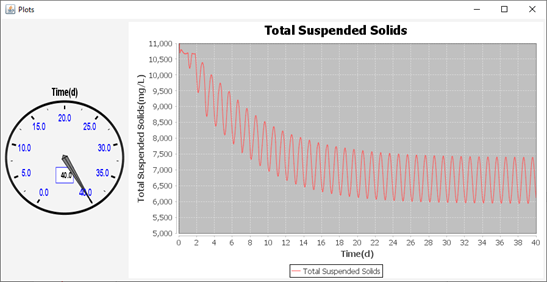
Figure 17‑7 – Non-Steady-State Python Script Output
20. Update the Python Script. We will now update the script so that it starts the simulation at steady state. Change the value fed to the gpsx.setSteady to True. Additionally, change the y-axis limits on the chart, defined by the rangeAxis.setRange(5000.0, 11000.0) command, such that the upper limit is 8,000 mg/L of total suspended solids.
21. Save the Python script.
22. Run the Python Script. Open the Python Script Manager. Run the script by pressing the Run Script button.
The results of the script can be seen in Figure 17‑8. The total suspended solids in the secondary clarifier recycle stream exhibits a sinusoidal pattern with constant maximum and minimum bounds. When this output is compared to the results of the previous Python script, it can be seen that the non-steady state simulations converges to the same output pattern as presented in the steady state simulation.
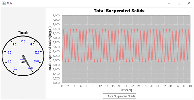
Figure 17‑8 - Steady State Test Python Script Output
Once a model has been calibrated, mathematical optimization can be employed to find the best operating conditions to achieve certain objectives such as minimizing net energy usage, total chemical usage or the overall operating costs. These objectives are directly impacted by numerous variables in the model which the user can set independently of the other variables in the model.
The Nelder-Mead Simplex method available in GPS-X is ideal when solving optimization problems with a small number of target and manipulated variables, but can be slow as the size of the problem increases. A Data Driven Optimization (DDO) Method has been included in the GPS-X install that is ideal for optimization with multiple parameters. The computational time of this method is largely independent of the number of manipulated parameters in the optimization problem but rather depends on the complexity of the model and the number of iterations desired.
In this tutorial, we will find the optimal operating conditions to minimize a plants net energy consumption under different operating conditions. We will be manipulating variables that have direct impact on the plants energy consumption well ensuring that the plant effluent quality is maintained within emission limits.
The purpose of this tutorial is to see how Python can be used to optimize the operating conditions used in GPS-X. By the end of this tutorial, you can use Python to solve complex optimization problems in a GPS-X layout.
The following emission limits and operational constraints have been imposed on our treatment plant and must be observed:
Table 18‑1 - Plant Effluent Limits
|
Effluent Constraint |
Lower Bound |
Upper Bound |
Units |
|
Total Suspended Solids |
0.0 |
20.0 |
mg/L |
|
Total Carbonaceous BOD5 |
0.0 |
10.0 |
mgO2/L |
|
Total Nitrogen |
0.0 |
7.5 |
mgN/L |
|
Ammonia Nitrogen |
0.0 |
0.2 |
mgN/L |
|
Ortho-Phoshate |
0.0 |
0.02 |
mgP/L |
Table 18‑2 - Plant Operational Constraints
|
Operational Constraint |
Lower Bound |
Upper Bound |
Units |
|
Mixed Liquor Suspended Solids |
1500.0 |
5000.0 |
mg/L |
We will now look at how custom GPS-X code can be used to create an objective function. Alternatively, this could be obtained directly in Python by collecting each variable in the objective function and directly calculating the objective function.
1. Load the starting point layout. We’ve already set up a layout to be used for this tutorial. The layout can be found at File > Sample Layouts > Tutorials> Tutorial 18 (Starting Point).
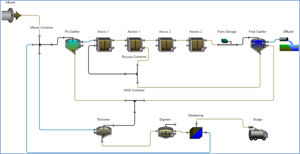
Figure 18‑1 - Tutorial 18 Layout
2. Save the Layoutwith a new name. We will be making changes to the layout and do not want to change the starting point layout.
3. Open the Macros User File. This can be opened by going to Layout > General Data > User Files > Macros…
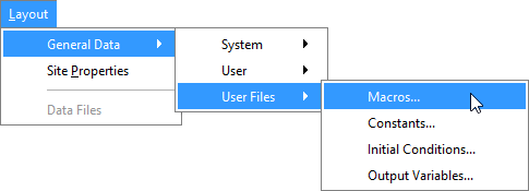
Figure 18‑2 - Accessing the Macro File
You will be adding code to the Derivative section of the Macro file.
4. Add Macro Code. You will be creating a single GPS-X variable to represent our objective function. Add the following code to the DERIVATIVE SECTION of the macro file to allow GPS-X to automatically calculate this variable.
netenergylayout = totalpowerkw - electricitySavedwdig/24.0
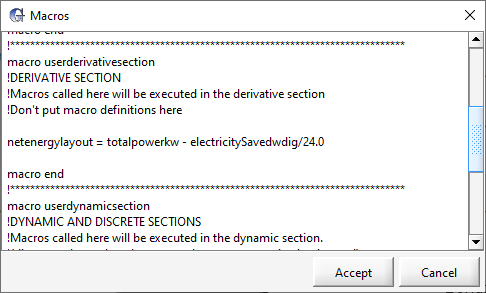
Figure 18‑3 - Updated Macro Code
The netenergylayout variable will be our optimization objective function. The calculation examines the difference between the instantaneous energy consumption (kW) in the plant and the estimated electricity that can be generated by the digester unit (kWh).
5. Click Accept in the Macros window to save the changes.
6. Create an Output Variable for the objective function. The custom Output Variables entry form can be found by going to Layout > General Data > User Files > Output Variables…
7. Add the following code to the output variable entry form:
display netenergylayout !Net Energy Used in the Layout !kW
8. Click Accept in the Output Variables window to save the changes.
9. Save the Layout and reload. This will cause GPS-X to read in the output variable and create a menu for it under Layout > General Data > User > Output Variables > User Defined Output Variables as displayed in Figure 18‑4.
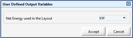
Figure 18‑4 - User Defined Output Variables Menu
10. Open Simulation Mode.
11. Create a Digital Type Output Graph containing the following variables:
· Layout > General Data > User > Output Variables > User Defined Output Variables > Net Energy used in the Layout
· Aerobic 2 effluent > Concentrations > Mixed Liquor Suspended Solids
· Effluent > Concentrations > Total Suspended Solids
· Effluent > Concentrations > total cBOD5
· Effluent > Concentrations > Ammonia Nitrogen
· Effluent > Concentrations > Total Nitrogen
· Effluent > Concentrations > Ortho-Phosphate
12. Run a 0-Day Steady State Simulation.This will allow you to see the baseline operation of the plant prior to preforming any optimization.
Notice in Figure 18‑5 how the plant is currently has a net energy usage of 15.26 kW well exceeding the limits for both Mixed Liquor suspended Solids and Ortho-Phosphate.
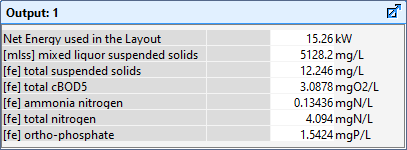
Figure 18‑5 – Unoptimized Outputs of a 0-Day Steady State Simulation
13. A Python script has already been created for use in this tutorial. Locate and open the Python script called ‘tutorial-18-0Day.py’. The Python script can be found in the following directory:
\layouts\08tutorials\
14. Save the Python Script. Save the script in the current working directory.
15. Add the Script to GPS-X. Open the Python Script Manager in GPS-X and add the Python script to GPS-X.
16. Edit the Script. Press the Edit button to open the script in Notepad. We will now discuss what the script is doing:
The ctypes Python library is used to interface the DDO and sobol_sampling functions found in a Dynamic Link Library (DLL) within the GPS-X instillation. Using the ctypes library, the input types of the ddo function have been defined using the data types available in the ctypes library.
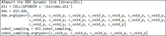
Figure 18‑6 - Adding the Dynamic Link Library Functions to the Python Script
Next, we define the optimization conditions to be used in the optimization:
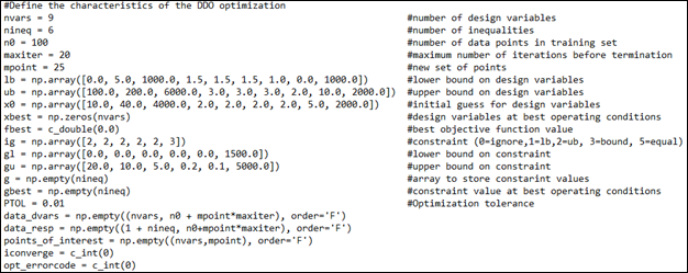
Figure 18‑7 – Optimization Problem Definition
· nvars – represents the number of target variables to be manipulated in the optimization. This is the number of inputs we will be changing in GPS-X
· nineq – represents the number of constraints in the optimization problem
· n0 – This is the number of points that will be used in the training set
· maxiter – This is the maximum number of optimizer iterations that can occur before the optimization is terminated
· lb – These are the lower bounds of the design variables
· ub – These are the upper bounds of the design variables
· x0 – These are the initial guesses to be used for the design variables
· xbest – This is a list that contains the design variable values that resulted in the best objective function value
· fbest – This variable contains the best objective function value
· gl – This is the lower bound of the constraints
· gu – This is the upper bound of the constraints
· ig – This represents the type of constraint that is being used. 0 indicates that the constraint can be ignored, 1 indicates that the constraint is a one-sided greater than or equal to constraint, 2 indicates that the constraint is a one-sided less than or equal to constraint, 3 indicates that it is a two-sided constraint, 5 represents that it is an equality constraint
· g – This is a list where the current value of the constrained variables are stored
· gbest – This is a list that contains the value of the constrained variables when using the design variables that resulted in the best objective function value
· data_dvars – A matrix that is used to contain the manipulated points to be tested
· data_resp – A matrix that contains the results of the tested conditions
· points_of_interest – Is a matrix of points that the ddo optimizer would like to investigate
· PTOL –Is the optimizer tolerance to be used for termination prior to reaching the maximum number of iterations
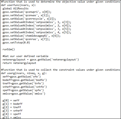
Figure 18‑8 - Functions to Set Input Values and Collect Outputs
The userfunc to set the current value of the design variables in GPS-X and start a simulation in GPS-X. The value of the objective function is collected at the end of the simulation and returned from the function.
The userg function collects the value of the constrained variables at the end of the 0-Day simulation.
17. Run the Script. Press the Run Script button with the script highlighted. The time required to run the script is affected by the speed of your workstation and the complexity of the model.
The best objective function value, the design variable values used to obtain it and the value of the constrained variables will be displayed in the output section of the Python Script Manager. The results of the 0-Day DDO optimization can be seen in Figure 18‑9.
Note: When using the DDO optimizer, ensure that you verify that a solution has been achieved that satisfies all of the constraints. The optimizer will not tell you if some constraints have not been met.
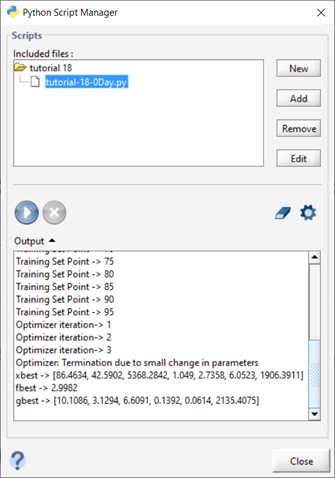
Figure 18‑9 - Results of the 0-Day DDO Optimization
18. Modify the Python Script. Change the value of n0 to 25, the value of maxiter to 5 and the value of mpoint to 7.
19. Save the Python Script.
20. Run the Script. This will illustrate the tradeoff between computational speed and optimizer performance that is faced when choosing the number of iterations that the optimizer will use. By decreasing the number of iterations used, a fesiable solution is obtain in less computational time but our objective function has increased by 2.12 kW. It is important to consider this tradeoff when constructing an optimization problem
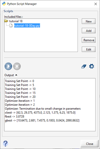
Figure 18‑10 - Results of the Modified 0-Day DDO Optimization
Well optimizing plant operation in a 0-Day simulation can help identify possible operational improvements, it only provides a snapshot of the actual plant operation. By preforming a dynamic simulation, you can determine parameter settings that are optimal over long periods of standard operating conditions or during extreme weather conditions. Python and GPS-X both allow you to insert real plant data into the simulation, allowing you to perform an optimization on real operating conditions experienced at your plant.
Note: When preforming DDO on Dynamic Data, the process can be very lengthy. The simulations in this section may take multiple hours to converge to a solution depending on the speed of your workstation.
21. A Python script has already been created for use with this section of the tutorial. Locate and open the Python script titled ‘tutorial-18-Dynamic.py’. The Python script can be found in the following directory:
\layouts\08tutorials\
22. Save the Python Script. Save the script in the current working directory
23. Add the Script to GPS-X. Open the Python Script Manager in GPS-X and add the Python script to GPS-X.
24. Edit the Script. Press the Edit button to open the script in Notepad. We will now discuss what has been changed from the ‘tutorial-18-0Day.py’ script:
The script has been modified to run a 1.0 day dynamic simulation. Due to the simulation being changed to a dynamic simulation, a communication interval will now occur in the simulation. A function, as seen in Figure 18‑11, will be called at each communication interval to collect the current value of the objection function variable and the constraints and add it to the cumulative sum. We will be minimizing the total net energy usage over the simulation period in this example.
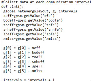
Figure 18‑11 - Function called at each Communication Interval in the Simulation
In this example, all of the collect constraint values are expected to exceed the bounds set in the 0-Day simulation as cumulative sums are now being collected rather than an instantaneous value. To accommodate this, we will constrain the average value of each constraint experienced across the communication interval. This is done by creating a variable which will track the number of communication intervals experienced during the simulation and dividing each element in array g by it. The code used to perform this average can be seen in Figure 18‑12.
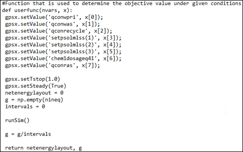
Figure 18‑12 - Updated userfunc Function that Averages the Constraint Values Collected in g
25. Create an Input controller for the Influent Flow type. This variable is accessed by right clicking on the Influent Object and going to Flow > FlowData.
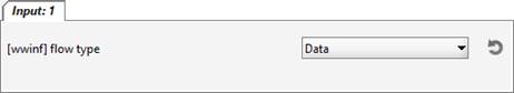
Figure 18‑13 - Influent Flow Type Controller
26. Using the input controller, set the influent flow type to Diurnal.
27. Run the Optimization Script.
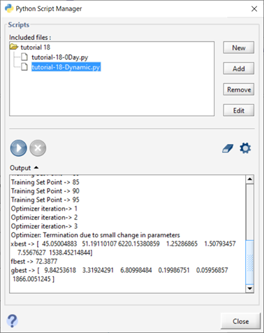
Figure 18‑14 - DDO Optimizer Output for a 1-Day Dynamic Simulation with Diurnal Influent Flow
28. After the simulation has finished, change the influent flow type to Sinusoidal and run the Script again. This will allow you to see the effects it has on the optimization results.
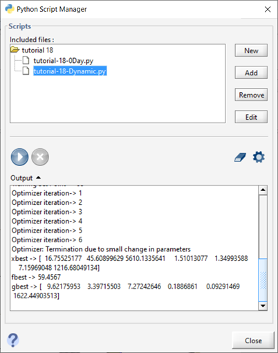
Figure 18‑15 - DDO Optimizer Output for a 1-Day Dynamic Simulation with Sinusoidal Influent Flow
[1] See GPS-X Technical Reference for more information on these Models
[2] Output variables are defined within each object and at each of the object's connection points
[3] The term static is used to describe the process of data input and output in this case in order to differentiate it from the case of input and output involving time series data which is described in Tutorial 4
[4] For the tuning mode to operate properly, the controller sampling time must be set to a reasonable value, e.g. the execution time of the controller to be implemented. This is why the controller sampling time was left as 0.05 days
[i] Reference: Marlin T.E., Process Control: Designing Processes and Control Systems for Dynamic Performance, McGraw-Hill, 1995